Z-transform done quick

August 26, 2012

The Z-transform is a standard tool in signal processing; however, most descriptions of it focus heavily on the mechanics of manipulation and don’t give any explanation for what’s going on. In this post, my goal is to cover only the basics (just enough to understand standard FIR and IIR filter formulations) but make it a bit clearer what’s actually going on. The intended audience is people who’ve seen and used the Z-transform before, but never understood why the terminology and notation is the way it is.

Polynomials

In an earlier draft, I tried to start directly with the standard Z-transform, but that immediately brings up a bunch of technicalities that make matters more confusing than necessary. Instead, I’m going to start with a simpler setting: let’s look at polynomials.

Not just any polynomials, mind. Say we have a finite sequence of real or complex numbers $a_0, \dots, a_n$ . Then we can define a corresponding polynomial that has the values in that sequence as its coefficients:

$\displaystyle A := \sum_{i=0}^n a_i x^i$ .

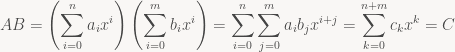
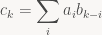
and of course there’s also a corresponding polynomial function A(x) that plugs in concrete values for x. Polynomials are closed under addition and scalar multiplication (both componentwise, or more accurately in this case, coefficient-wise) so they are a vector space and we can form linear combinations $\lambda A + \mu B$ . That’s reassuring, but not particularly interesting. What is interesting is the other fundamental operation we can do with polynomials: Multiply them. Let’s say we multiply two polynomials A and B to form a third polynomial C, and we want to find the corresponding coefficients:

$\displaystyle AB = \left( \sum_{i=0}^n a_i x^i \right) \left( \sum_{i=0}^m b_i x^i \right) = \sum_{i=0}^n \sum_{j=0}^m a_i b_j x^{i+j} = \sum_{k=0}^{n+m} c_k x^k = C$ .

To find the coefficients of C, we simply need to sum across all the combinations of indices i, j such that i+j=k, which of course means that j=k-i:

$\displaystyle c_k = \sum_i a_i b_{k-i}$ .

When I don’t specify a restriction on the summation index, that simply means “sum over all i for which the right-hand side is well-defined”. And speaking of notation, in the future, I don’t want to give a name to every individual expression just so we can look at the coefficients; instead, I’ll just write $[x^k]\ AB$ to denote the coefficient of x^k in the product of A and B – which is of course our c_k. Anyway, this is simply the discrete convolution of the two input sequences, and we’re gonna milk this connection for all it’s worth.

Knowing nothing but this, we can already do some basic filtering in this form if we want to: Suppose our a_i encode a sampled sound effect. A again denotes the corresponding polynomial, and let’s say $B = (1 + x)$ , corresponding to the sequence (1, 1). Then C=AB computes the convolution of A with the sequence (1, 1), i.e. each sample and its immediate successor are summed (this is a simple but unnormalized low-pass filter). Now so far, we’ve only really substituted one way to write convolution for another. There’s more to the whole thing than this, but for that we need to broaden our setting a bit.

Generating functions

The next step is to get rid of the fixed-length limitation. Instead of a finite sequence, we’re now going to consider potentially infinite sequences $(a_i)_{i=0}^\infty$ . A finite sequence is simple one where all but finitely many of the a_i are zero. Again, we can create a corresponding object that captures the whole sequence – only instead of a polynomial, it’s now a power series:

$\displaystyle A := \sum_{i=0}^\infty a_i x^i$ .

And the corresponding function A(x) is called a_i‘s generating function. Now we’re dealing with infinite series, so if we want to plug in an actual value for x, we have to worry about convergence issues. For the time being, we won’t do so, however; we simply treat the whole thing as a formal power series (essentially, an “infinite-degree polynomial”), and all the manipulations I’ll be doing are justified in that context even if the corresponding series don’t converge.

Anyway, the properties described above carry over: we still have linearity, and there’s a multiplication operation (the Cauchy product) that is the obvious generalization of polynomial multiplication (in fact, the formula I’ve written above for the c_k still applies) and again matches discrete convolution. So why did I start with polynomials in the first place if everything stays pretty much the same? Frankly, mainly so I don’t have to whip out both infinite sequences and power series in the second paragraph; experience shows that when I start an article that way, the only people who continue reading are the ones who already know everything I’m talking about anyway. Let’s see whether my cunning plan works this time.

So what do we get out of the infinite sequences? Well, for once, we can now work on infinite signals – or, more usually, signals with a length that is ultimately finite, but not known in advance, as occurs with real-time processing. Above we saw a simple summing filter, generated from a finite sequence. That sequence is the filter’s “impulse response”, so called because it’s the result you get when applying the filter to the unit impulse signal (1 0 0 …). (The generating function corresponding to that signal is simply “1”, so this shouldn’t be much of a surprise). Filters where the impulse response has finite length are called “finite impulse response” or FIR filters. These filters have a straight-up polynomial as their generating function. But we can also construct filters with an infinite impulse response – IIR filters. And those are the filters where we actually get something out of going to generating functions in the first place.

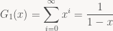
Let’s look at the simplest infinite sequence we can think of: (1 1 1 …), simply an infinite series of ones. The corresponding generating function is

$\displaystyle G_1(x) = \sum_{i=0}^\infty x^i$

And now let’s look at what we get when we convolve a signal a_i with this sequence:

$\displaystyle s_k := [x^k]\ A G_1(x) = \sum_{i=0}^k a_i \cdot 1 = \sum_{i=0}^k a_i$

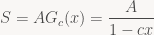
Expanding out, we see that s₀ = a₀, s₁ = a₀ + a₁, s₂ = a₀ + a₁ + a₂ and so forth: convolution with G₁ generates a signal that, at each point in time, is simply the sum of all values up to that time. And if we actually had to compute things this way, this wouldn’t be very useful, because our filter would keep getting slower over time! Luckily, G₁ isn’t just an arbitrary function – it’s a geometric series, which means that for concrete values x, we can compute G₁(x) as:

$\displaystyle G_1(x) = \sum_{i=0}^\infty x^i = \frac{1}{1 - x}$

and more generally, for arbitrary $c \ne 0$

$\displaystyle G_c(x) = \sum_{i=0}^\infty (cx)^i = \sum_{i=0}^\infty c^i x^i = \frac{1}{1 - cx}$ .

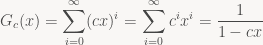
If we apply the identity the other way round, we can turn such an expression of x back into a power series; in particular, when dealing with formal power series, the left-hand side is the definition of the expression on the right-hand side. This notation also suggests that G₁ is the inverse (wrt. convolution) of (1 – x), and more generally that G_c is the inverse of (1 – cx). Verifying this makes for a nice exercise.

But what does that mean for us? It means that, given the expression

$\displaystyle S = A G_c(x) = \frac{A}{1 - cx}$

we can treat it as the identity between power series that it is and multiply both sides by (1 – cx), giving:

$\displaystyle S (1 - cx) = A$

and thus

$\displaystyle [x^k]\ S (1 - cx) = s_k - c s_{k-1} = a_k \Leftrightarrow s_k = a_k + c s_{k-1}$

i.e. we can compute s_k in constant time if we’re allowed to look at s_k-1. In particular, for the c=1 case we started with, this just means the obvious thing: don’t throw the partial sum away after every sample, instead just keep adding the most recent sample to the running total.

And here’s the thing: that’s everything you need to compute convolutions with almost any sequence that has a rational generating function, i.e. it’s a quotient of polynomials $P(x) / Q(x)$ . Using the same trick as above, it’s easy to see what that means computationally. Say that $P(x) = p_0 + p_1 x + \cdots + p_n x^n$ and $Q(x) = q_0 + q_1 x + \cdots + q_m x^m$ . If our signal has the generating function A(x), then computing the filtered signal S boils down to evaluating $S(x) := A(x) P(x) / Q(x)$ . Along the same lines as before, we have

$\displaystyle [x^k]\ S (q_0 + q_1 x + \cdots + q_m x^m) = [x^k] A (p_0 + \cdots + p_n x^n)$

$\displaystyle \Leftrightarrow q_0 s_k + q_1 s_{k-1} + \cdots + q_m s_{k-m} = p_0 a_k + \cdots + p_n a_{k-n}$

$\displaystyle \Leftrightarrow q_0 s_k = \left(\sum_{j=0}^n p_j a_{k-j}\right) - \left(\sum_{j=1}^m q_j s_{k-j}\right)$

$\displaystyle \Rightarrow s_k = \frac{1}{q_0} \left(\sum_{j=0}^n p_j a_{k-j} - \sum_{j=1}^m q_j s_{k-j}\right)$ .

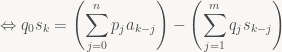
So again, we can compute the signal incrementally using a fixed amount of work (depending only on n and m) for every sample, provided that q₀ isn’t zero. The question is, do these rational functions still have a corresponding series expansion? After all, this is what we need to employ generating functions in the first place. Luckily, the answer is yes, again provided that q₀ isn’t zero. I’ll skip describing how exactly this works since we’ll be content to deal directly with the factored rational function form of our generating functions from here on out; if you want more details (and see just how useful the notion of a generating function turns out to be for all kinds of problems!), I recommend you look at the excellent “Concrete Mathematics” by Graham, Knuth and Patashnik or the by now freely downloadable “generatingfunctionology” by Wilf.

At last, the Z-transform

At this point, we already have all the theory we need for FIR and IIR filters, but with a non-standard notation, motivated by the desire to make the connection to standard polynomials and generating functions more explicit. Let’s fix that up: in signal processing, it’s customary to write a signal x as a function $x : \mathbb{Z} \rightarrow \mathbb{R}$ (or $x : \mathbb{Z} \rightarrow \mathbb{C}$ ), and it’s customary to write the argument in square brackets. So instead of dealing with sequences that consist of elements x_n, we now have functions with values at integer locations x[n]. And the (unilateral) Z-transform of our signal x is now the function

$\displaystyle X(z) = \mathcal{Z}(x) = \sum_{n=0}^{\infty} x[n] z^{-n}$ .

in other words, it’s basically a generating function, but this time the exponents are negative. I also assume that the signal is x[n] = 0 for all n<0, i.e. the signal starts at some defined point and we move that point to 0. This doesn’t make any fundamental difference for the things I’ve discussed so far: all the properties discussed above still hold, and indeed all the derivations will still work if you mechanically substitute x^k with z^-k. In particular, anything involving convolutions still works exactly same. However it does make a difference if you actually plug in concrete values for z, which we are about to do. Also note that our variable is now z, not x. Customarily, “z” is used to denote complex variables, and this is no exception – more in a minute. Next, the Z-transform of our filter’s impulse response (which is essentially the filter’s generating function, except now we evaluate at 1/z) is called the “transfer function” and has the general form

$\displaystyle H(z) = \frac{P(z^{-1})}{Q(z^{-1})} = \frac{Y(z)}{X(z)}$

where P and Q are the same polynomials as above; these polynomials in z^-1 are typically written Y(z) and X(z) in the DSP literature. You can factorize the numerator and denominator polynomials to get the zeroes and poles of a filter. They’re important concepts in IIR filter design, but fairly incidental to what I’m trying to do (give some intution about what the Z-transform does and how it works), so I won’t go into further detail here.

The Fourier connection

One last thing: The relation of this all to frequency space, or: what do our filters actually do to frequencies? For this, we can use the discrete-time Fourier transform (DTFT, not to be confused with the Discrete Fourier Transform or DFT). The DTFT of a general signal x is

$\displaystyle \hat{X}(\omega) = \sum_{n=-\infty}^{\infty} x[n] e^{-i\omega n}$

Now, in our case we’re only considering signals with x[n]=0 for n<0, so we get

$\displaystyle \hat{X}(\omega) = \sum_{n=0}^\infty x[n] e^{-i\omega n} = \sum_{n=0}^\infty x[n] \left(e^{i\omega}\right)^{-n} = X(e^{i\omega})$

which means we can compute the DTFT of a signal by evaluating its Z-transform at exp(iω) – assuming the corresponding series of expression converges. Now, if the Z-transform of our signal is in general series form, this is just a different notation for the same thing. But for our rational transfer functions H(z), this is a big deal, because evaluating their values at given complex z is easy – it’s just a rational function, after all.

In fact, since we know that polynomial (and series) multiplication corresponds to convolution, we can now also easily see why convolution filters are useful to modify the frequency response (Fourier transform) of a signal: If we have a signal x with Z-transform X and the transfer function of a filter H, we get:

$\displaystyle (X \cdot H)(e^{i\omega}) = X(e^{i\omega}) H(e^{i\omega})$

and in particular

$\displaystyle |(X \cdot H)(e^{i\omega})| = |X(e^{i\omega})| |H(e^{i\omega})|$

The first of these two equations is the discrete-time convolution theorem for Fourier transforms of signals: the DTFT of the convolution of the two signals is the point-wise product of the DTFTs of the original signal and the filter. The second shows us how filters can amplify or attenuate individual frequencies: if |H(e^iω)| > 1, frequency ω will be amplified in the filtered signal, and it it’s less than 1, it will be dampened.

Conclusion and further reading

The purpose of this post was to illustrate a few key concepts and the connections between them:

Polynomial/series multiplication and convolution are the same thing.
The Z-transform is very closely related to generating functions, an extremely powerful technique for manipulating sequences.
In particular, the transfer function of a filter isn’t just some arbitrary syntactic convention to tie together the filter coefficients; there’s a direct connection to corresponding sequence manipulations.
The Fourier transform of filters is directly tied to the behavior of H(z) in the complex plane; computing the DTFT of an IIR filter’s impulse response directly would get messy, but the factored form of H(z) makes it easy.
With this background, it’s also fairly easy to see why filters work in the first place.

I intentionally cover none of these aspects deeply; my experience is that most material on the subject does a great job of covering the details, at the expense of making it harder to see the big picture, so I wanted to try doing it the other way round. More details on series and generating functions can be found in the two books I cited above, and a good introduction to digital filters that supplies the details I omitted is Smith’s Introduction to Digital Filters.

From → Maths

4 Comments

atyuwen permalink

Great article. But there is a typo in the last formula of the section ”Generating functions”, check the parentheses.

Reply
- fgiesen permalink
  
  Where? I don’t see anything.
  
  Reply
atyuwen permalink

The Eq.
s_k = \frac{1}{q_0}\left(\sum_{j=0}^n{p_ja_{k-j}}\right)-\left(\sum_{j=1}^m{q_js_{k-j}}\right)
should be
s_k = \frac{1}{q_0}\left(\sum_{j=0}^n{p_ja_{k-j}}-\sum_{j=1}^m{q_js_{k-j}}\right)

Reply
- fgiesen permalink
  
  Ah, yes, of course you’re right :). Thanks, fixed.
  
  Reply

Z-transform done quick

Polynomials

Generating functions

At last, the Z-transform

The Fourier connection

Conclusion and further reading

Leave a reply to atyuwen Cancel reply

Recent Posts

Categories

Archives

Z-transform done quick

Polynomials

Generating functions

At last, the Z-transform

The Fourier connection

Conclusion and further reading

Share this:

Related

Leave a reply to atyuwen Cancel reply

Recent Posts

Categories

Archives