A string processing rant

This post is part of a series – go here for the index.

Rants are not usually the style of this blog, but this one I just don’t want to keep in. So if you’re curious, the actual information content of this post will be as follows: C string handling functions kinda suck. So does C++’s std::string. Dealing with wide character strings using only standard C/C++ functionality is absolutely horrible. And VC++’s implementation of said functionality is a damn minefield. That’s it. You will not actually learn anything more from reading this post. Continue at your own risk.

UPDATE: As “cmf” points out in the comments, there are actually C++ functions that seem to do what I wanted in the first place with a minimum amount of fuss. Goes to show, the one time I post a rant on this blog and of course I’m wrong! :) That said, I do stand by my criticism of the numerous API flaws I point out in this post, and as I point out in myreply, the discoverability of this solution is astonishingly low; when I ran into this problem originally, not being familiar with std::wstring I googled a bit and checked out Stack Overflow and several other coding sites and mailing list archives, and what appears to be the right solution showed up on none of the pages I ran into. So at the very least I’m not alone. Ah well.

The backstory

I spent most of last weekend playing around with my fork of Intel’s Software Occlusion Culling sample. I was trying to optimize some of the hot spots, a process that involves a lot of small (or sometimes not-so-small) modifications to the code followed by a profiling run to see if they help. Now unfortunately this program, at least in its original version, had loading times of around 24 seconds on my machine, and having to wait for those 24 seconds every time before you can even start the profiling run (which takes another 10-20 seconds if you want useful results) gets old fast, so I decided to check whether there was a simple way to shorten the load times.

Since I already had the profiler set up, I decided to take a peek into the loading phase. The first big time-waste I found was a texture loader that was unnecessarily decompressing a larger DXT skybox texture, and then recompressing it again. I won’t go into details here; suffice it to say that once I had identified the problem, it was straightforward enough to fix, and it cut down loading time to about 12 seconds.

My next profiling run showed me this:

I’ve put a red dot next to functions that are called either directly or indirectly by the configuration-file class CPUTConfigFile. Makes you wonder, doesn’t it? Lest you think I’m exaggerating, here’s some of the call stacks for our #2 function, malloc:

Here’s the callers to #5, free:

And here’s memcpy, further down:

I have to say, I’ve done optimization work on lots of projects over the years, and it’s rare that you’ll see a single piece of functionality leave a path of destruction this massive in its wake. The usual patterns you’ll see are either “localized performance hog” (a few functions completely dominating the profile, like I saw in the first round with the texture loading) or the “death by a thousand paper cuts”, where the profile is dominated by lots of “middle-man” functions that let someone else do the actual work but add a little overhead each time. As you can see, that’s not what’s going on here. What we have here is the rare “death in all directions” variant. Why settle for paper cuts, just go straight for the damn cluster bomb!

At this point it was clear that the whole config file thing needed some serious work. But first, I was curious. Config file loading and config block handling, sure. But what was that RemoveWhitespace function doing there? So I took a look.

How not to remove whitespace

Let’s cut straight to the chase: Here’s the code.

void RemoveWhitespace(cString &szString)
{
    // Remove leading whitespace
    size_t nFirstIndex = szString.find_first_not_of(_L(' '));
    if(nFirstIndex != cString::npos)
    {
        szString = szString.substr(nFirstIndex);
    }

    // Remove trailing newlines
    size_t nLastIndex = szString.find_last_not_of(_L('\n'));
    while(nLastIndex != szString.length()-1)
    {
        szString.erase(nLastIndex+1,1);
        nLastIndex = szString.find_last_not_of(_L('\n'));
    };
    // Tabs
    nLastIndex = szString.find_last_not_of(_L('\t'));
    while(nLastIndex != szString.length()-1)
    {
        szString.erase(nLastIndex+1,1);
        nLastIndex = szString.find_last_not_of(_L('\t'));
    };
    // Spaces
    nLastIndex = szString.find_last_not_of(_L(' '));
    while(nLastIndex != szString.length()-1)
    {
        szString.erase(nLastIndex+1,1);
        nLastIndex = szString.find_last_not_of(_L(' '));
    };
}

As my current and former co-workers will confirm, I’m generally a fairly calm, relaxed person. However, in moments of extreme frustration, I will (on occasion) perform a “*headdesk*”, and do so properly.

This code did not drive me quite that far, but it was a close call.

Among the many things this function does wrong are:

• While it’s supposed to strip all leading and trailing white space (not obvious from the function itself, but clear in context), it will only trim leading spaces. So for example leading tabs won’t get stripped, nor will any spaces that follow after those tabs.
• The function will remove trailing spaces, tabs, and newlines – provided they occur in exactly that order: first all spaces, then all tabs, then all newlines. But the string “test\t \n” will get trimmed to “test\t” with the tab still intact, because the tab-stripping loop will only tabs that occur at the end of the string after the newlines have been removed.
• It removes white space characters it finds front to back rather than back to front. Because of the way C/C++ strings work, this is an O(N²) operation. For example, take a string consisting only of tabs.
• The substring operation creates an extra temporary string; while not horrible by the standards of what else happens in this function, it’s now becoming clear why RemoveWhitespace manages to feature prominently in the call stacks for malloc, free and memcpy at the same time.
• And let’s not even talk about how many times the string is scanned from front to back.

That by itself would be bad enough. But it turns out that in context, not only is this function badly implemented, most of the work it does is completely unnecessary. Here’s one of its main callers, ReadLine:

CPUTResult ReadLine(cString &szString, FILE *pFile)
{
    // TODO: 128 chars is a narrow line.  Why the limit?
    // Is this not really reading a line, but instead just reading the next 128 chars to parse?
    TCHAR   szCurrLine[128] = {0};
    TCHAR *ret = fgetws(szCurrLine, 128, pFile);
    if(ret != szCurrLine)
    {
        if(!feof(pFile))
        {
            return CPUT_ERROR_FILE_ERROR;
        }
    }

    szString = szCurrLine;
    RemoveWhitespace(szString);

    // TODO: why are we checking feof twice in this loop?
    // And, why are we using an error code to signify done?
    // eof check should be performed outside ReadLine()
    if(feof(pFile))
    {
        return CPUT_ERROR_FILE_ERROR;
    }

    return CPUT_SUCCESS;
}

I’ll let the awesome comments speak for themselves – and for the record, no, this thing really is supposed to read a line, and the ad-hoc parser that comes after this will get out of sync if it’s ever fed a line with more than 128 characters in it.

But the main thing of note here is that szString is assigned from a C-style (wide) string. So the sequence of operations here is that we’ll first allocate a cString (which is a typedef for a std::wstring, by the way), copy the line we read into it, then call RemoveWhitespace which might create another temporary string in the substr call, to follow it up with several full-string scans and possibly memory moves.

Except all of this is completely unnecessary. Even if we need the output to be a cString, we can just start out with a subset of the C string to begin with, rather than taking the whole thing. All RemoveWhitespace really needs to do is tell us where the non-whitespace part of the string begins and ends. You can either do this using C-style string handling or, if you want it to “feel more C++”, you can express it by iterator manipulation:

static bool iswhite(int ch)
{
    return ch == _L(' ') || ch == _L('\t') || ch == _L('\n');
}

template
static void RemoveWhitespace(Iter& start, Iter& end)
{
    while (start < end && iswhite(*start))
        ++start;

    while (end > start && iswhite(*(end - 1)))
        --end;
}

Note that this is not only much shorter, it also correctly deals with all types of white space both at the beginning and the end of the line. Instead of the original string assignment we then do:

    // TCHAR* obeys the iterator interface, so...
    TCHAR* start = szCurrLine;
    TCHAR* end = szCurrLine + tcslen(szCurrLine);
    RemoveWhitespace(start, end);
    szString.assign(start, end);

Note how I use the iterator range form of assign to set up the string with a single copy. No more substring operations, no more temporaries or O(N²) loops, and after reading we scan over the entire string no more than two times, one of those being in tcslen. (tcslen is a MS extension that is the equivalent of strlen for TCHAR – which might be either plain char or wchar_t, depending on whether UNICODE is defined – this code happens to be using “Unicode”, that is, UTF-16).

There’s only two other calls to RemoveWhitespace, and both of these are along the same vein as the call we just saw, so they’re just as easy to fix up.

Problem solved?

Not quite. Even with the RemoveWhitespace insanity under control, we’re still reading several megabytes worth of text files with short lines, and there’s still between 1 and 3 temporary string allocations per line in the code, plus whatever allocations are needed to actually store the data in its final location in the CPUTConfigBlock.

Long story short, this code still badly needed to be rewritten to do less string handling, so I did. My new code just reads the file into a memory buffer in one go (the app in question takes 1.5GB of memory in its original form, we can afford to allocate 650K for a text file in one block) and then implements a more reasonable scanner that processes the data in place and doesn’t do any string operations until we need to store values in their final location. Now, because the new scanner assumes that ASCII characters end up as ASCII, this will actually not work correctly with some character encodings such as Shift-JIS, where ASCII-looking characters can appear in the middle of encodings for multibyte characters (the config file format mirrors INI files, so ‘[‘, ‘]’ and ‘=’ are special characters, and the square brackets can appear as second characters in a Shift-JIS sequence). It does however still work with US-ASCII text, the ISO Latin family and UTF-8, which I decided was acceptable for a config file reader. I did still want to support Unicode characters as identifiers though, which meant I was faced with a problem: once I’ve identified all the tokens and their extents in the file, surely it shouldn’t be hard to turn the corresponding byte sequences into the std::wstring objects the rest of the code wants using standard C++ facilities? Really, all I need is a function with this signature:

void AssignStr(cString& str, const char* begin, const char* end);

Converting strings, how hard can it be?

Turns out: quite hard. I could try using assign on my cString again. That “works”, if the input happens to be ASCII only. But it just turns each byte value into the corresponding Unicode code point, which is blatantly wrong if our input text file actually has any non-ASCII characters in it.

Okay, so we could turn our character sequence into a std::string, and then convert that into a std::wstring, never mind the temporaries for now, we can figure that out later… wait, WHAT? There’s actually no official way to turn a string containing multi-byte characters into a wstring? How moronic is that?

Okay, whatever. Screw C++. Just stick with C. Now there actually is a standard function to convert multi-byte encodings to wchar_t strings, and it’s called, in the usual “omit needless vowels” C style, mbstowcs. Only that function can’t be used on an input string that’s delimited by two pointers! Because while it accepts a size for the output buffer, it assumes the input is a 0-terminated C string. Which may be a reasonable protocol for most C string-handling functions, but is definitely problematic for something that’s typically used for input parsing, where you generally aren’t guaranteed to have NUL characters in the right places.

But let’s assume for a second that we’re willing to modify the input data (const be damned) and temporarily overwrite whatever is at end with a NUL character so we can use mbstowcs – and let me just remark at this point that awesomely, the Microsoft-extended safe version of mbstowcs, mbstowcs_s, accepts two arguments for the size of the output buffer, but still doesn’t have a way to control how many input characters to read – if you decide to extend a standard API anyway, why can’t you fix it at the same time? Anyway, if we just patch around in the source string to make mbstowcs happy, does that help us?

Well, it depends on how loose you’re willing to play with the C++ standard. The goal of the whole operation was to reduce the number of temporary allocations. Well, mbstowcs wants a wchar_t output buffer, and writes it like it’s a C string, including terminating NUL. std::wstring also has memory allocated, and normal implementations will store a terminating 0 wchar_t, but as far as I can tell, this is not actually guaranteed. In any case, there’s a problem, because we need to reserve the right number of wchar’s in the output string, but it’s not guaranteed to be safe to do this:

void AssignStr(cString& str, const char* begin, const char* end)
{
    // patch a terminating NUL into *end
    char* endPatch = (char*) end;
    char oldEnd = *end;
    *endPatch = 0;

    // mbstowcs with NULL arg counts how many wchar_t's would be
    // generated
    size_t numOut = mbstowcs(NULL, begin, 0);

    // make sure str has the right size
    str.resize(numOut, ' ');

    // convert characters including terminating NUL and hope it's
    // going to be OK?
    mbstowcs(&str[0], begin, numOut + 1);

    // restore the original end
    *endPatch = oldEnd;
}

This might work, or it might not. As far as I know, it would be legal for a std::wstring implementation to only append a trailing NUL character lazily whenever c_str() is first called on a particular string. Either way, it’s fairly gross. I suppose I could resize to numOut + 1 elements, and then later do another resize after the mbstowcs is done; that way should definitely be safe.

Either way is completely beside the point though. This is an actual, nontrivial operation on strings that is a totally reasonable thing to do, and that the C IO system will in fact do for me implicitly if I use fgetws. Why are all the functions dealing with this so horribly broken for this use case that’s not at all fancy? Did anyone ever look at this and decide that it was reasonable to expect people to write code like this? WHAT THE HELL?

It gets better

That’s not it quite yet, though. Because when I actually wrote the code (as opposed to summarizing it for this blog post), I didn’t think to patch in the NUL byte on the source string. So I went for the alternative API that works character by character: the C function mbtowc. Now, awesomely, because it works character by character, and is not guaranteed to see all characters in a multi-byte sequence in the same call, it has to keep state around of which partial multi-byte sequences it has seen to be able to decode characters. So it’s not thread-safe, and POSIX defines an extended version mbrtowc that makes you pass in a pointer to that state which does make it thread-safe. At this point though, I don’t care about thread-safety (this code is single-threaded anyway), and besides, in our case I actually know that the characters between begin and end are supposed to parse correctly. So I just don’t worry about it. Also, instead of actually counting the right number of wchar_t‘s ahead of time in a second pass, I just assume that the string is generally likely to have less wide characters than the source multi-byte string has bytes. Even if that turns out wrong (which won’t happen for conventional encodings), the std::wstring we write to can dynamically resize, so there’s not much that can go wrong. So I ended up with this implementation:

void AssignStr(cString& dest, const char* begin, const char* end)
{
    dest.clear();
    if (end <= begin)
        return;

    size_t len = end - begin;
    size_t initial = len + 1; // assume most characters are 1-byte
    dest.reserve(initial);

    const char* p = start;
    while (p < end)
    {
        wchar_t wc;
        int len = mbtowc(&wc, p, end - p);
        if (len < 1) // NUL byte or error
            break;

        p += len;
        dest.push_back(wc);
    }
}

Looks fairly reasonable, right?

Well, one profiling session later, I noticed that performance had improved, but it turned out that I was apparently wrong to assume that, like its std::vector counterpart, std::wstring::push_back would basically compile into the moral equivalent of dest.data[dest.len++] = wc. Instead, what I saw in VTune (with a kind of morbid fascination) was about two dozen instructions worth of inlined insanity surrounding a call to std::wstring::insert. For every character. In a release build.

It’s probably the VC++ STL doing something stupid. At this point, I don’t feel like investigating why this is happening. Whatever, I’m just gonna add some more to this layer cake of insanity. Just stop thinking and start coding. So I figure that hey, if adding stuff to strings is apparently an expensive operation, well, let’s amortize it, eh? So I go for this:

void AssignStr(cString& dest, const char* begin, const char* end)
{
    dest.clear();
    if (end <= begin)
        return;

    static const int NBUF = 64;
    wchar_t buf[NBUF];
    int nb = 0;

    size_t len = end - begin;
    size_t initial = len + 1; // assume most characters are 1-byte
    dest.reserve(initial);

    const char* p = start;
    while (p < end)
    {
        int len = mbtowc(&buf[nb++], p, end - p);
        if (len < 1) // NUL byte or error
            break;

        p += len;
        if (p >= end || nb >= NBUF)
        {
            dest.append(buf, buf + nb);
            nb = 0;
        }
    }
}

And it’s still slow, and I still get a metric ton of bullshit inlined for that call. Turns out this happens because I call the general “input iterator” variant of append which, go figure, adds character by character. Silly me! What I really should’ve called is dest.append(buf, nb). Of course! Once I figure that one out, I profile again, and sure enough, this time there’s no magic std::string functions cluttering up the profile anymore. Finally. Mission accomplished, right?

Not so fast, bucko.

Ohhh no. No, there’s one final “surprise” waiting for me. I put surprise in quotes because we already saw it in my first profile screenshot.

Yeah right. Those C functions we’ve been calling? In the VC++ C runtime library, all of them end up calling a constructor for a C++ object for some reason.

No, I’m not gonna comment on that one. I stopped caring a few paragraphs ago. Go ahead, put C++ code in your C runtime library. Whatever makes you happy.

So it turns out that VC++ has two versions of all the multibyte conversion functions: one that uses the current locale (which you can query using _get_current_locale()) and one that takes an explicit locale_t parameter. And if you don’t pass in a locale yourself, mbtowc and so forth will call _get_current_locale() themselves, and that ends up calling a C++ constructor for some reason. (I don’t care, I’m in my happy place right now. La la la).

And I finally decide to screw portability – hey, it’s a VC++-only project anyway – and call _get_current_locale() once, pass it to all my calls, and the magic constructor disappears, and with it the last sign of dubious things happening in the string handling.

Hooray.

Conclusions

So, what do we have here: we have a C++ string class that evidently makes it easy to write horrendously broken code without noticing it, and simultaneously doesn’t provide some core functionality that apps which use both std::wstring and interface with non-UTF16 character sets (which is almost nobody, I’m sure!) will need. We have C functions that go out of their way to make it hard to use them correctly. We have the Microsoft camp that decides that the right way to fix these functions is to fix buffer overflows, and we have the POSIX camp that decides that the right way to fix them is to fix the race condition inherent in their global state. Both of these claim that their modifications are more important than the other’s, and then there’s the faction that holds the original C standard library to be the only true way, ignoring the fact that this API is clearly horribly broken no matter how you slice it. Meanwhile, std::wstring gets another attention fix by making it unnecessarily hard to actually get data from C APIs into it without extra copying (and may I remind you that I’m only using C APIs here because there doesn’t seem to be an official C++ API!), while the VC++ standard library proves its attention deficit by somehow making a push_back to a properly pre-allocated string an expensive operation. And for the final act of our little performance, watch as a constructor gets called from C code, a veritable Deus Ex Machina that I honestly didn’t see coming.

As my friend Casey Muratori would put it: Everyone is fired.

And now excuse me while I apply some bandages and clean the blood off my desk.

Write combining is not your friend

This post is part of a series – go here for the index.

Most memory you deal with on a daily basis is cached; on CPUs, it’s usually write-back cached. While dealing with processor caches can be counter-intuitive, caching works well most of the time, and it’s mostly transparent to the programmer (and certainly the user). However, if we are to use the cache to service memory reads, we need to make sure to invalidate our cache entries if someone else writes to the corresponding memory locations. This is implemented using one of several mechanisms referred to as “coherency protocols”, which CPU cores use to synchronize their caches with each other.

That is not the subject of this post, though. Because while such mechanisms are in place for CPUs talking to each other, there is nothing equivalent for the CPU talking to other non-CPU devices, such as GPUs, storage or network devices. Generally, communication with such devices still happens via system memory (or by memory-mapping registers or device memory so they appear to be system memory, which doesn’t make much difference from the CPU core’s point of view), but the CPU is not going to be notified of changes in a timely fashion, so normal caching is out.

Originally, device memory used to be accessed completely without caching. That’s safe (or at least as safe as it’s going to get) but also slow, because each memory access gets turned into an individual bus transaction, which has considerable overhead. Now anything related to graphics tends to move a lot of data around. Before widespread hardware acceleration, it was mostly the CPU writing pixels to the frame buffer, but now there’s other graphics-related writes too. So finally we get write combining, where the CPU treats reads as uncached but will buffer writes for a while in the hope of being able to combine multiple adjacent writes into a larger bus transaction. This is much faster. Common implementations have much weaker memory ordering guarantees than most memory accesses, but that’s fine too; this kind of thing tends to be used mainly for bulk transfers, where you really don’t care in which order the bytes trickle into memory. All you really want is some mechanism to make sure that all the writes are done before you pull the trigger and launch a command buffer, display a frame, trigger a texture upload, whatever.

All this is fairly straightforward and reasonable. However, the devil’s in the details, and in practice write combining is finicky. It’s really easy to make a small mistake that results in a big performance penalty. I’ve seen this twice in the last two days, on two different projects, so I’ve decided to write up some guidelines.

Where is write combining used?

I’m only going to talk about graphics here. For all I know, write-combining might be used for lots of other things, but I would assume that even if that is true, graphics is the only mainstream application where WC memory is exposed to user-mode applications.

So the main way to get a pointer to write-combining memory is by asking a 3D or GPGPU API to map a buffer or texture into memory: that is, using GL glMapBuffer, D3D9 Lock, CL clEnqueueMap* or D3D1x Map. Not all such buffers are write-combined, but those used for rapid uploads usually are – doubly so if you’re requesting a “write-only” mapping, which all mentioned APIs support.

What happens if you read from write-combined memory?

Sadly, the answer is not “reading from write-combined memory isn’t allowed”. This would be much simpler and less error-prone, but at least on x86, the processor doesn’t even have the notion of memory that can be written but not read.

Instead, what actually happens is that the read is treated as uncached. This means all pending write-combining buffers get flushed, and then the read is performed without any cache. Flushing write-combining buffers costs time and results in stores of partial cache lines, which is also inefficient. And of course uncached reads are really slow too.

Don’t read from write-combining memory, unless you have a very good reason to (you probably don’t). In particular, never read values back from constant buffers, vertex buffers or index buffers you’re currently writing to. Ever.

How bad can it possibly be? Let me show you an example. Here’s an excerpt of a VTune profile for an application I recently looked at:

As you can see, a lot of time is being spent in CPUTModelDX11::SetRenderStates. Worse, as VTune helpfully highlights for us, this function runs at an absolutely appalling 9.721 clock cycles per instruction (CPI Rate)! Now it turns out that a large fraction is due to these innocent-looking lines that write to a constant buffer:

    pCb = (CPUTModelConstantBuffer*)mapInfo.pData;
    pCb->World               = world;
    pCb->ViewProjection      = view * projection;
    pCb->WorldViewProjection = world * pCb->ViewProjection;

Note how pCb->ViewProjection is used as an argument for a matrix multiply in the last line. Now, here’s the simple fix:

    XMMATRIX viewProj = view * projection;
    pCb = (CPUTModelConstantBuffer*)mapInfo.pData;
    pCb->World               = world;
    pCb->ViewProjection      = viewProj;
    pCb->WorldViewProjection = world * viewProj;

And here’s the corresponding VTune profile:

Now, this profile was somewhat longer so the actual cycle counts are different, but the point stands: This simple change made the function drop from the #5 to the #12 spot, and based on the CPI rate, it now runs more than twice as fast per invocation – mind you, 4.4 cycles/instruction is still pretty bad, but it’s certainly an improvement over the 9.7 we saw earlier.

Other things to be careful about

Okay, so not reading is an important point. What else? Well, it depends on the processor. Early x86s had fairly restrictive rules about write combining: writes had to be of certain sizes, they needed to be properly aligned, and accesses needed to be purely sequential. The first two can be dealt with, but the latter is tricky when dealing with C/C++ compilers that try to move schedule writes for optimum efficiency. For several years, it used to be that you basically had to mark all pointers to vertex buffers etc. as volatile to make sure the compiler didn’t try to reorder writes and inadvertently break write-combining in the process. While not as bad as reads, this still results in a very noticeable drop in performance.

Luckily, x86 processors from about 2002 on are far more tolerant about writes arriving out of order and will generally be able to combine writes even if they’re not perfectly sequential. However, other processors (such as those found in some game consoles) aren’t as tolerant; better safe than sorry. And even if you don’t strictly need to enforce sequential accesses, it’s still a good idea to write the code that way, because of the next rule:

Avoid holes. If you’re writing to a memory range, write the whole range. If you’re writing a dynamic vertex buffer, write every field, even if your shader ignores some of them. If you map a buffer, write the whole thing – even if you (think you) know some of the contents don’t need to change. Any hole will break the sequence and turn what would otherwise be one large write into at least two smaller ones. On some processors, it has other adverse effects too. That’s why you want to write struct fields sequentially, at least in your source code – that way, it’s easier to check against the struct definition to make sure you left nothing out.

Conclusion

Write combining is a powerful technique to accelerate writes to graphics memory, but it’s very easy to misuse in a way that causes severe performance degradation. Worse, because things only get slow but don’t crash, such problems can creep in and not be noticed for a long time. Short of profiling your code periodically, there’s little you can do to find them. Here’s the summary:

• If it’s a dynamic constant buffer, dynamic vertex buffer or dynamic texture and mapped “write-only”, it’s probably write-combined.
• Never read from write-combined memory.
• Try to keep writes sequential. This is good style even when it’s not strictly necessary. On processors with picky write-combining logic, you might also need to use volatile or some other way to cause the compiler not to reorder instructions.
• Don’t leave holes. Always write large, contiguous ranges.
• Check the rules for your target architecture. There might be additional alignment and access width limitations.

If you live by these rules, write-combining can be a powerful ally in writing high-performance graphics code. But never a friend – it will stab you in the back on the first opportunity. So be careful.

Order-preserving bijections

Sometimes it’s useful to convert numbers to a different representation in a way that’s order-preserving. This is useful because some applications have a clear preference for one type of number over another – for example, Radix sort and the closely related Radix trees are most naturally expressed in terms of unsigned integers, and it’s generally easier to transform the keys so they sort correctly as unsigned ints than it is to adapt the algorithm to deal with signed numbers (or floats).

Another case of interest is SIMD instructions on x86. For example, there’s signed integer greater-than comparison instructions PCMPGTB, PCMPGTW and PCMPGTD starting with the Pentium MMX (or SSE2 for 128-bit variants), but no unsigned equivalents. There’s also signed word integer min/max PMINSW and PMAXSW starting from SSE (SSE2 for 128-bit), but for some reason the corresponding unsigned equivalents PMINUW and PMAXUW weren’t added until SSE4.1.

So, without further ado, here’s my transforms of choice (assuming two’s complement arithmetic):

Signed int32 <-> unsigned int32

• x ^= 0x80000000;
• or: x += 0x80000000;
• or: x -= 0x80000000;

All three do the same thing and are involutions (i.e. they are their own inverse).

Mnemonic: To convert signed integers to unsigned integers, add 0x80000000 so the smallest signed integer (-0x80000000) turns into the smallest unsigned integer (0). The same works in reverse of course.

The MSB doesn’t carry into anything, so addition and exclusive or do the same thing. Note that 0x80000000 isn’t a representable integer in 32-bit two’s complement arithmetic, but -0x80000000 is, so technically the correct expressions are x -= -0x80000000 instead of x += 0x80000000 (and similar for subtraction), but you get the idea. This generalizes to integers with other sizes in the obvious way.

IEEE float <-> signed int32

Float to int32:

int32 temp   = float2bits(f32_val);
int32 i32val = temp ^ ((temp >> 31) & 0x7fffffff);

int32 to float:

int32 temp   = i32val ^ ((i32val >> 31) & 0x7fffffff);
float f32val = bits2float(temp);

Aside from the “bit casting” (turn an IEEE754 float number into its integer bits and back) this transform is an involution too. It uses bit shifts on signed two’s complement numbers which is technically undefined in C, but in practice all compilers I’ve ever used just turn it into the arithmetic right shifts you’d expect.

Positive floats have the MSB (integer sign bit) clear and larger floating-point values have larger integer representations. This includes the IEEE infinity value, which is larger than all finite floats. Negative floats have the MSB (integer sign bit) set, but they are represented as sign + magnitude, so 0x800000 actually represents the largest “negative” float (actually, it’s -0), whereas smaller (more negative) floats have larger representations when compared as integers. This expression leaves positive floats alone but flips all but the sign bit for negative floats, so they order correctly.

Caveat 1: Under this transform, -0 < 0, whereas "true" IEEE comparisons treat them as the same.
Caveat 2: There’s NaNs (not a number) both with and without the sign bit set. Under this transform, the “smallest” and “largest” values can both represent NaN bit patterns, and NaNs are ordered relative to each other. This is well-defined and reasonable, but doesn’t match the behavior or regular floating-point compares.

IEEE float <-> unsigned int32

Float to uint32:

uint32 temp   = float2bits(f32_val);
uint32 i32val = temp ^ (((int32)temp >> 31) | 0x80000000);

uint32 to float:

int32  temp1  = u32val ^ 0x80000000;
int32  temp2  = temp1 ^ (temp1 >> 31);
float  f32val = bits2float(temp2);

This is really just a combination of the previous two: instead of making sure we don’t change the sign bit, we make sure to always flip it in the forward transform. Because we flip the sign, the reverse transform needs to flip it back before it does the arithmetic shift, so this is not an involution unlike the other two. The same caveats apply as for the int32 version.

Min, Max under negation and an AABB trick

The two obvious identities:

min(a,b) = -max(-a, -b)
max(a,b) = -min(-a, -b)

can be used to rewrite algorithms using mixed min/max expressions in terms of just min (or just max). This can sometimes be useful when working with data that is intended to be processed with SIMD instructions, because it can be used to make the dataflow more regular. Let me give you a simple example to show what I mean: computing the axis-aligned bounding box (or AABB for short) of the union of several 2D AABBs.

AABB of the union of N 2D AABBs

A common representation for a 2D AABB just stores the extrema in both X and Y:

union AlignedBox2 {
  struct {
    float min_x, min_y;
    float max_x, max_y;
  };
  Vec4 simd;
};

The AABB for the union of N such AABBs can then be computed by computing the min/max over all bounds in the array, as follows:

AlignedBox2 union_bounds(const AlignedBox2 *boxes, int N) // N >= 1
{
  AlignedBox2 r = boxes[0];
  for (int i=1; i < N; i++) {
    r.min_x = min(r.min_x, boxes[i].min_x);
    r.min_y = min(r.min_y, boxes[i].min_y);
    r.max_x = max(r.max_x, boxes[i].max_x);
    r.max_y = max(r.max_y, boxes[i].max_y);
  }
  return r;
}

A typical 4-wide SIMD implementation can apply the operations to multiple fields at the same time, but ends up wasting half the SIMD lanes on fields it doesn’t care about, and does some extra work at the end to merge the results back together:

AlignedBox2 union_bounds_simd(const AlignedBox2 *boxes, int N)
{
  Vec4 mins = boxes[0].simd;
  Vec4 maxs = boxes[0].simd;
  for (int i=1; i < N; i++) {
    mins = min(mins, boxes[i].simd);
    maxs = max(maxs, boxes[i].simd);
  }

  AlignedBox2 r;
  r.minx = mins[0]; // or equivalent shuffle...
  r.miny = mins[1];
  r.maxx = maxs[2];
  r.maxy = maxs[3];
  return r;
}

But the identities above suggest that it might help to use a different (and admittedly somewhat weird) representation for 2D boxes instead, where we store the negative of max_x and max_y:

union AlignedBox2b {
  struct {
    float min_x, min_y;
    float neg_max_x, neg_max_y;
  };
  Vec4 simd;
};

If we write the computation of the union bounding box of two AABBs A and B in this form, we get (the interesting part only):

  r.min_x = min(a.min_x, b.min_x);
  r.min_y = min(a.min_y, b.min_y);
  r.neg_max_x = min(a.neg_max_x, b.neg_max_x);
  r.neg_max_y = min(a.neg_max_y, b.neg_max_y);

where the last two lines are just the result of applying the identity above to the original computation of max_x / max_y (with all the sign flips thrown in). Which means the SIMD version in turn becomes much easier (and doesn’t waste any work anymore):

AlignedBox2b union_bounds_simd(const AlignedBox2b *boxes, int N)
{
  AlignedBox2b r = boxes[0];
  for (int i=1; i < N; i++)
    r.simd = min(r.simd, boxes[i]);

  return r;
}

And the same approach works for intersection too – in fact, all you need to do to get a box intersection function is to turn the min into a max.

Now, this is just a toy example, but it shows the point nicely – sometimes a little sign flip can go a long way. In particular, this trick can come in handy when dealing with 3D AABBs and the like, because groups of 3 don’t fit nicely in typical SIMD vector sizes, and you don’t always have another float-sized value to sandwich in between; even if you don’t store the negative of the max, it’s usually much easier to sign-flip individual lanes than it is to rearrange them.

Small note on Quaternion distance metrics

There’s multiple ways to measure distances between unit quaternions (a popular rotation representation in 3D). What’s interesting is that the popular choices are essentially all equivalent.

Polar form

A standard way to build quaternions is using the polar (axis-angle) form
, where n is the (unit length) axis of rotation, θ is the angle, and i, j and k are the imaginary basis vectors.

For a rotation in this form, we know how “far” it goes: it’s just the angle θ. Since the real component of q is just cos(θ/2), we can read off the angle as

where the dot denotes the quaternion dot product.

This measures, in a sense, how far away the quaternion is from the identity element 1. To get a distance between two unit quaternions q and r, we rotate both of them such that one of them becomes the identity element. To do this for our pair q, r, we simply multiply both by r’s inverse from the left, and since r is a unit quaternion its inverse and conjugate are the same:

Note that cosine is a monotonic function over the interval we care about, so in any numerical work, there’s basically never the need to actually calculate that arc cosine: instead of checking, say, whether the angle is less than some maximum error threshold T, we can simple check that the dot product is larger than cos(T/2). If you’re actually taking the arc cosine for anything other than display purposes, you’re likely doing something wrong.

Dot product

Another way is to use the dot product directly as a distance measure between two quaternions. How does this relate to the angle from the polar form? It’s the same, as we quickly find out when we use the fact that the dot product is invariant under rotations:

and hence also

So again, whether we minimize the angle between q and r (as measured in the polar form) or maximize the dot product between q and r boils down to the same thing. But there’s one final choice left.

L₂ distance

The third convenient metric is just using the norm of the difference between the two quaternions: . The question is, can we relate this somehow to the other two? We can, and as is often the case, it’s easier to work with the square of the norm:

.

In other words, the distance between two unit quaternions again just boils down to the dot product between them – albeit with a scale and bias this time.

Conclusion

The popular choices of distance metrics between quaternions all boil down to the same thing. The relationships between them are simple enough that it’s easy to convert, say, an exact error bound on the norm between two quaternions into an exact error bound on the angle of the corresponding rotation. Each of these three representations is the most convenient to use in some context; feel free to convert back and forth between them for different solvers; they’re all compatible in the sense that their minima will always agree.

UPDATE: As Sam points out in the comments, you need to be careful about the distinction between quaternions and rotations here (I cleared up the language in the article slightly). Each rotation in 3-dimensional real Euclidean space has two representations as a quaternion: the quaternion group double-covers the rotation group. If you want to measure the distances between rotations not quaternions, you need to use slightly modified metrics (see his comment for details).

Frustum planes from the projection matrix

Another quick one. Now this is another old trick, but it’s easy to derive and still not as well-known as it deserves to be, so here goes.

All modern graphics APIs ultimately expect vertex coordinates to end up in one common coordinate system where clipping is done – clip space. That’s the space that vertices passed to the rasterizer are expected in – and hence, the space that Vertex Shaders (or Geometry Shaders, or Domain/Tessellation Evaluation Shaders) transform to. These shaders can do what they want, but the usual setup matches the original fixed-function pipeline and splits vertex transformations into at least two steps: The projection transform and the model-view transform, both of which can be represented as homogeneous 4×4 matrices.

The projection transform is the part that transforms vertices from camera view space to clip space. A view-space input vertex position v is transformed with the projection matrix P and gives us the position of the vertex in clip space:

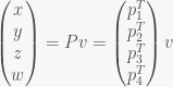
Here, I’ve split P up into its four row vectors p₁^T, …, p₄^T. Now, in clip space, the view frustum has a really simple form, but there’s two slightly different formulations in use. GL uses the symmetric form:

whereas D3D replaces the last row with . Either way, we get 6 distinct inequalities, each of which corresponds to exactly one clip plane: is the left clip plane, is the right clip plane, and so forth. Now from the equation above we know that and and hence

Or in words, v lies in the non-negative half-space defined by the plane p₄^T+p₁^T – we have a view-space plane equation for the left frustum plane! For the right plane, we similarly get

and in general, for the GL-style frustum we find that the six frustum planes in view space are exactly the six planes p₄^T±p_i^T for i=1, 2, 3 – all you have to do to get the plane equations is to add (or subtract) the right rows of the projection matrix! For a D3D-style frustum, the near plane is different, but it takes the even simpler form , so it’s simply defined by the third row of the projection matrix.

Deriving frustum planes from your projection matrix in this way has the advantage that it’s nice and general – it works with any projection matrix, and is guaranteed to agree with the clipping / culling done by the GPU, as long as the planes are in fact derived from the projection matrix used for rendering.

And if you need the frustum planes in some other space, say in model space: not too worry! We didn’t use any special properties of P – the derivation works for any 4×4 matrix. The planes obtained this way are in whatever space the input matrix transforms to clip space – in the case of P, view space, but it can be anything. To give an example, if you have a model-view matrix M, then PM is the combined matrix that takes us from model-space to clip-space, and extracting the planes from PM instead of P will result in model-space clip planes.

Z-transform done quick

The Z-transform is a standard tool in signal processing; however, most descriptions of it focus heavily on the mechanics of manipulation and don’t give any explanation for what’s going on. In this post, my goal is to cover only the basics (just enough to understand standard FIR and IIR filter formulations) but make it a bit clearer what’s actually going on. The intended audience is people who’ve seen and used the Z-transform before, but never understood why the terminology and notation is the way it is.

Polynomials

In an earlier draft, I tried to start directly with the standard Z-transform, but that immediately brings up a bunch of technicalities that make matters more confusing than necessary. Instead, I’m going to start with a simpler setting: let’s look at polynomials.

Not just any polynomials, mind. Say we have a finite sequence of real or complex numbers . Then we can define a corresponding polynomial that has the values in that sequence as its coefficients:

.

and of course there’s also a corresponding polynomial function A(x) that plugs in concrete values for x. Polynomials are closed under addition and scalar multiplication (both componentwise, or more accurately in this case, coefficient-wise) so they are a vector space and we can form linear combinations . That’s reassuring, but not particularly interesting. What is interesting is the other fundamental operation we can do with polynomials: Multiply them. Let’s say we multiply two polynomials A and B to form a third polynomial C, and we want to find the corresponding coefficients:

.

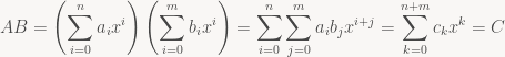
To find the coefficients of C, we simply need to sum across all the combinations of indices i, j such that i+j=k, which of course means that j=k-i:

.

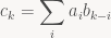
When I don’t specify a restriction on the summation index, that simply means “sum over all i for which the right-hand side is well-defined”. And speaking of notation, in the future, I don’t want to give a name to every individual expression just so we can look at the coefficients; instead, I’ll just write to denote the coefficient of x^k in the product of A and B – which is of course our c_k. Anyway, this is simply the discrete convolution of the two input sequences, and we’re gonna milk this connection for all it’s worth.

Knowing nothing but this, we can already do some basic filtering in this form if we want to: Suppose our a_i encode a sampled sound effect. A again denotes the corresponding polynomial, and let’s say , corresponding to the sequence (1, 1). Then C=AB computes the convolution of A with the sequence (1, 1), i.e. each sample and its immediate successor are summed (this is a simple but unnormalized low-pass filter). Now so far, we’ve only really substituted one way to write convolution for another. There’s more to the whole thing than this, but for that we need to broaden our setting a bit.

Generating functions

The next step is to get rid of the fixed-length limitation. Instead of a finite sequence, we’re now going to consider potentially infinite sequences . A finite sequence is simple one where all but finitely many of the a_i are zero. Again, we can create a corresponding object that captures the whole sequence – only instead of a polynomial, it’s now a power series:

.

And the corresponding function A(x) is called a_i‘s generating function. Now we’re dealing with infinite series, so if we want to plug in an actual value for x, we have to worry about convergence issues. For the time being, we won’t do so, however; we simply treat the whole thing as a formal power series (essentially, an “infinite-degree polynomial”), and all the manipulations I’ll be doing are justified in that context even if the corresponding series don’t converge.

Anyway, the properties described above carry over: we still have linearity, and there’s a multiplication operation (the Cauchy product) that is the obvious generalization of polynomial multiplication (in fact, the formula I’ve written above for the c_k still applies) and again matches discrete convolution. So why did I start with polynomials in the first place if everything stays pretty much the same? Frankly, mainly so I don’t have to whip out both infinite sequences and power series in the second paragraph; experience shows that when I start an article that way, the only people who continue reading are the ones who already know everything I’m talking about anyway. Let’s see whether my cunning plan works this time.

So what do we get out of the infinite sequences? Well, for once, we can now work on infinite signals – or, more usually, signals with a length that is ultimately finite, but not known in advance, as occurs with real-time processing. Above we saw a simple summing filter, generated from a finite sequence. That sequence is the filter’s “impulse response”, so called because it’s the result you get when applying the filter to the unit impulse signal (1 0 0 …). (The generating function corresponding to that signal is simply “1”, so this shouldn’t be much of a surprise). Filters where the impulse response has finite length are called “finite impulse response” or FIR filters. These filters have a straight-up polynomial as their generating function. But we can also construct filters with an infinite impulse response – IIR filters. And those are the filters where we actually get something out of going to generating functions in the first place.

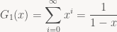
Let’s look at the simplest infinite sequence we can think of: (1 1 1 …), simply an infinite series of ones. The corresponding generating function is

And now let’s look at what we get when we convolve a signal a_i with this sequence:

Expanding out, we see that s₀ = a₀, s₁ = a₀ + a₁, s₂ = a₀ + a₁ + a₂ and so forth: convolution with G₁ generates a signal that, at each point in time, is simply the sum of all values up to that time. And if we actually had to compute things this way, this wouldn’t be very useful, because our filter would keep getting slower over time! Luckily, G₁ isn’t just an arbitrary function – it’s a geometric series, which means that for concrete values x, we can compute G₁(x) as:

and more generally, for arbitrary

.

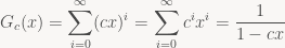
If we apply the identity the other way round, we can turn such an expression of x back into a power series; in particular, when dealing with formal power series, the left-hand side is the definition of the expression on the right-hand side. This notation also suggests that G₁ is the inverse (wrt. convolution) of (1 – x), and more generally that G_c is the inverse of (1 – cx). Verifying this makes for a nice exercise.

But what does that mean for us? It means that, given the expression

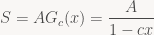
we can treat it as the identity between power series that it is and multiply both sides by (1 – cx), giving:

and thus

i.e. we can compute s_k in constant time if we’re allowed to look at s_k-1. In particular, for the c=1 case we started with, this just means the obvious thing: don’t throw the partial sum away after every sample, instead just keep adding the most recent sample to the running total.

And here’s the thing: that’s everything you need to compute convolutions with almost any sequence that has a rational generating function, i.e. it’s a quotient of polynomials . Using the same trick as above, it’s easy to see what that means computationally. Say that and . If our signal has the generating function A(x), then computing the filtered signal S boils down to evaluating . Along the same lines as before, we have

.

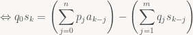
So again, we can compute the signal incrementally using a fixed amount of work (depending only on n and m) for every sample, provided that q₀ isn’t zero. The question is, do these rational functions still have a corresponding series expansion? After all, this is what we need to employ generating functions in the first place. Luckily, the answer is yes, again provided that q₀ isn’t zero. I’ll skip describing how exactly this works since we’ll be content to deal directly with the factored rational function form of our generating functions from here on out; if you want more details (and see just how useful the notion of a generating function turns out to be for all kinds of problems!), I recommend you look at the excellent “Concrete Mathematics” by Graham, Knuth and Patashnik or the by now freely downloadable “generatingfunctionology” by Wilf.

At last, the Z-transform

At this point, we already have all the theory we need for FIR and IIR filters, but with a non-standard notation, motivated by the desire to make the connection to standard polynomials and generating functions more explicit. Let’s fix that up: in signal processing, it’s customary to write a signal x as a function (or ), and it’s customary to write the argument in square brackets. So instead of dealing with sequences that consist of elements x_n, we now have functions with values at integer locations x[n]. And the (unilateral) Z-transform of our signal x is now the function

.

in other words, it’s basically a generating function, but this time the exponents are negative. I also assume that the signal is x[n] = 0 for all n<0, i.e. the signal starts at some defined point and we move that point to 0. This doesn’t make any fundamental difference for the things I’ve discussed so far: all the properties discussed above still hold, and indeed all the derivations will still work if you mechanically substitute x^k with z^-k. In particular, anything involving convolutions still works exactly same. However it does make a difference if you actually plug in concrete values for z, which we are about to do. Also note that our variable is now z, not x. Customarily, “z” is used to denote complex variables, and this is no exception – more in a minute. Next, the Z-transform of our filter’s impulse response (which is essentially the filter’s generating function, except now we evaluate at 1/z) is called the “transfer function” and has the general form

where P and Q are the same polynomials as above; these polynomials in z^-1 are typically written Y(z) and X(z) in the DSP literature. You can factorize the numerator and denominator polynomials to get the zeroes and poles of a filter. They’re important concepts in IIR filter design, but fairly incidental to what I’m trying to do (give some intution about what the Z-transform does and how it works), so I won’t go into further detail here.

The Fourier connection

One last thing: The relation of this all to frequency space, or: what do our filters actually do to frequencies? For this, we can use the discrete-time Fourier transform (DTFT, not to be confused with the Discrete Fourier Transform or DFT). The DTFT of a general signal x is

Now, in our case we’re only considering signals with x[n]=0 for n<0, so we get

which means we can compute the DTFT of a signal by evaluating its Z-transform at exp(iω) – assuming the corresponding series of expression converges. Now, if the Z-transform of our signal is in general series form, this is just a different notation for the same thing. But for our rational transfer functions H(z), this is a big deal, because evaluating their values at given complex z is easy – it’s just a rational function, after all.

In fact, since we know that polynomial (and series) multiplication corresponds to convolution, we can now also easily see why convolution filters are useful to modify the frequency response (Fourier transform) of a signal: If we have a signal x with Z-transform X and the transfer function of a filter H, we get:

and in particular

The first of these two equations is the discrete-time convolution theorem for Fourier transforms of signals: the DTFT of the convolution of the two signals is the point-wise product of the DTFTs of the original signal and the filter. The second shows us how filters can amplify or attenuate individual frequencies: if |H(e^iω)| > 1, frequency ω will be amplified in the filtered signal, and it it’s less than 1, it will be dampened.

Conclusion and further reading

The purpose of this post was to illustrate a few key concepts and the connections between them:

• Polynomial/series multiplication and convolution are the same thing.
• The Z-transform is very closely related to generating functions, an extremely powerful technique for manipulating sequences.
• In particular, the transfer function of a filter isn’t just some arbitrary syntactic convention to tie together the filter coefficients; there’s a direct connection to corresponding sequence manipulations.
• The Fourier transform of filters is directly tied to the behavior of H(z) in the complex plane; computing the DTFT of an IIR filter’s impulse response directly would get messy, but the factored form of H(z) makes it easy.
• With this background, it’s also fairly easy to see why filters work in the first place.

I intentionally cover none of these aspects deeply; my experience is that most material on the subject does a great job of covering the details, at the expense of making it harder to see the big picture, so I wanted to try doing it the other way round. More details on series and generating functions can be found in the two books I cited above, and a good introduction to digital filters that supplies the details I omitted is Smith’s Introduction to Digital Filters.

Quaternion differentiation

I wanted to point someone to a short explanation of this today and noticed, with some surprise, that I couldn’t find something concise within 5 minutes of googling. So it seems worth writing up. I’m assuming you know what quaternions are and what they’re used for.

First, though, it seems important to point one thing out: Actually, there’s nothing special at all about either integration or differentiation of quaternion-valued functions. If you have a quaternion-valued function of one variable q(t), then

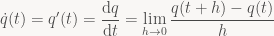
same as for any real- or complex-valued function.

So what, then, is this post about? Simple: unit quaternions are commonly used to represent rotations (or orientation of rigid bodies), and rigid-body dynamics require integration of orientation over time. Almost all sources I could find just magically pull a solution out of thin air, and those that give a derivation tend to make it way more complicated than necessary. So let’s just do this from first principles. I’m assuming you know that multiplying two unit quaternions quaternions q₁q₀ gives a unit quaternion representing the composition of the two rotations. Now say we want to describe the orientation q(t) of a rigid body rotating at constant angular velocity. Then we can write

where describes the rotation the body undergoes in one time step. Since we have constant angular velocity, we will have , and more generally for all nonnegative integer k by induction. So for even more general t we’d expect something like

.

Now, q_ω is a unit quaternion, which means it can be written in polar form

where θ is some angle and n is a unit vector denoting the axis of rotation. That part is usually mentioned in every quaternion tutorial. Embedding real 3-vectors as the corresponding pure imaginary quaternion, i.e. writing just for the quaternion , is usually also mentioned somewhere. What usually isn’t mentioned is the crucial piece of information that the polar form of a quaternion, in fact, just the quaternion version of Euler’s formula: Any unit complex number can be written as the complex exponential of a pure imaginary number , and similarly any unit-length quaternion (and q_ω in particular) can be written as the exponential of a pure imaginary quaternion

which gives us a natural definition for

.

Now, what if we want to write a differential equation for the behavior of q(t) over time? Just compute the derivative of q(t) as you would for any other function of t. Using the chain and product rules we get:

Now t and θ are real numbers, so the exponential is of a real number times n; exp is defined as a power series, and for arbitrary c real we have

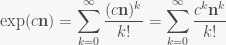
n commutes with powers of n, and real numbers commute with everything; therefore, n commutes with exp(cn) for arbitrary c, and thus

The vector θn is in fact just the angular velocity ω, which yields the oft-cited but seldom-derived equation:

This is usually quoted completely without context. In particular, it’s not usually mentioned that q(t) describes the orientation of a body with constant angular velocity, and similar for the crucial link to the exponential function.

Linear interpolation past, present and future

Linear interpolation. Lerp. The bread and butter of graphics programming. Well, turns out I have three tricks about lerps to share. One of them is really well known, the other two less so. So let’s get cracking!

Standard linear interpolation is just lerp(t, a, b) = (1-t)*a + t*b. You should already know this. At t=0 we get a, at t=1 we get b, and for inbetween values of t we interpolate linearly between the two. And of course we can also linearly extrapolate by using a t outside [0,1].

Past

The expression shown above has two multiplies. Now, it used to be the case that multiplies were really slow (and by the way they really aren’t anymore, so please stop doubling the number of adds in an expression to get rid of a multiply, no matter what your CS prof tells you). If multiplies are expensive, there’s a better (equivalent) expression you can get with some algebra: lerp(t, a, b) = a + t*(b-a). This is the first of the three tricks, and it’s really well known.

But in this setting (int multiplies are slow) you’re also really unlikely to have floating-point hardware, or to be working on floating-point numbers. Especially if we’re talking about pixel processing in computer graphics, it used to be all-integer for a really long time. It’s more likely to be all fixed-point, and in the fixed-point setting you typically have something like fixedpt_lerp(t, a, b) = a + ((t * (b-a)) >> 8). And more importantly, your a’s and b’s are also fixed-point (integer) numbers, typically with a very low range.

So here comes the second trick: for some applications (e.g. cross fades), you’re doing a lot of lerps with the same t (at least one per pixel). Now note that if t is fixed, the (t * (b - a)) >> 8 part really only depends on b-a, and that’s a small set of possible values: If a and b are byte values in [0,255], then d=b-a is in [-255,255]. So we really only ever need to do 511 multiplies based on t, to build a table indexed by d. Except that’s not true either, because we compute first t*0 then t*1 then t*2 and so forth, so we’re really just adding t every time, and we can build the whole table without any multiplies at all. So here we get trick two, for doing lots of lerps with constant t on integer values:

U8 lerp_tab[255*2+1]; // U8 is sufficient here

// build the lerp table
for (int i=0, sum = 0; i < 256; i++, sum += t) {
  lerp_tab[255-i] = (U8) (-sum >> 8); // negative half of table
  lerp_tab[255+i] = (U8) ( sum >> 8); // positive half
}

// cross-fade (grayscale image here for simplicity)
for (int i=0; i < npixels; i++) {
  int a = src1[i];
  int b = src2[i];
  out[i] = a + lerp_tab[255 + b-a];
}

Look ma, no multiplies!

Present

But back to the present. Floating-point hardware is readily available on most platforms and purely counting arithmetic ops is a poor estimator for performance on modern architectures. Practically speaking, for almost all code, you’re never going to notice any appreciable difference in speed between the two versions

  lerp_1(t, a, b) = (1 - t)*a + t*b
  lerp_2(t, a, b) = a + t*(b-a)

but you might notice something else: unlike the real numbers (which our mathematical definition of lerp is based on) and the integers (which our fixed-point lerps worked on), floating-point numbers don’t obey the arithmetic identities we’ve been using to derive this. In particular, for two floating point numbers we generally have a + (b-a) != b, so the second lerp expression is generally not correct at t=1! In contrast, with IEEE floating point, the first expression is guaranteed to return the exact value of a (b) at t=0 (t=1). So there’s actually some reason to prefer the first expression in that case, and using the second one tends to produce visible artifacts for some applications (you can also hardcode your lerp to return b exactly at t=1, but that’s just ugly and paying a data-dependent branch to get rid of one FLOP is a bad idea). While for pixel values you’re unlikely to care, it generally pays to be careful for mesh processing and the like; using the wrong expression can produce cracks in your mesh.

So what to do? Use the first form, which has one more arithmetic operation and does two multiplies, or the second form, which has one less operation but unfavorable rounding properties? Luckily, this dilemma is going away.

Future

Okay, “future” is stretching a bit here, because for some platforms this “future” started in 1990, but I digress. Anyway, in the future we’d like to have a magic lerp instruction in our processors that solves this problem for us (and is also fast). Unfortunately, that seems very unlikely: Even GPUs don’t have one, and Michael Abrash never could get Intel to give him one either. However, he did get fused multiply-adds, and that’s one thing all GPUs have too, and it’s either already on the processor you’re using or soon coming to it. So if fused multiply-adds can help, then maybe we’re good. And it turns out they can.

A fused multiply-add is just an operation fma(a, b, c) = a*b + c that computes the inner expression using only one exact rounding step. And FMA-based architectures tend to compute regular adds and multiplies using the same circuitry, so all three operations cost roughly the same (in terms of latency anyway, not necessarily in terms of power). And while I say “fma” these chips usually support different versions with sign flips in different places too (implementing this in the HW is almost free); the second most important one is “fused negative multiply-subtract”, which does fnms(a, b, c) = -(a*b - c) = c - a*b. Let’s rewrite our lerp expressions using FMA:

  lerp_1(t, a, b) = fma(t, b, (1 - t)*a)
  lerp_2(t, a, b) = fma(t, b-a, a)

Both of these still have arithmetic operations left that aren’t in FMA form; lerp_1 has two leftover ops and lerp_2 has one. And so far both of them aren’t significantly better than their original counterparts. However, lerp_1 has exactly one multiply and one subtract left; they’re just subtract-multiply (which we don’t have HW for), rather than multiply-subtract. However, that one is easily remedied with some algebra: (1 - t)*a = 1*a - t*a = a - t*a, and that last expression is in fma (more accurately, fnms) form. So we get a third variant, and our third trick:

  lerp_3(t, a, b) = fma(t, b, fnms(t, a, a))

Two operations, both FMA-class ops, and this is based on lerp_1 so it’s actually exact at the end points. Two dependent ops – as long as we don’t actually get a hardware lerp instruction, that’s the best we can hope for. So this version is both fast and accurate, and as you migrate to platforms with guaranteed FMA support, you should consider rewriting your lerps that way – it’s the lerp of the future!

Polynomials from repeated linear interpolation

It’s fairly well-known that Bezier curves can be evaluated using repeated linear interpolation – de Casteljau’s algorithm. It’s also fairly well-known that a generalization of this algorithm can be used to evaluate B-Splines: de Boor’s algorithm. What’s not as well known is that it’s easy to construct interpolating polynomials using a very similar approach, leading to an algorithm that is, in a sense, halfway between the two.

In the following, I’ll write for linear interpolation. I’ll stick with quadratic curves since they are the lowest-order curves to show “interesting” behavior for the purposes of this article; everything generalizes to higher degrees in the obvious way.

De Casteljau’s algorithm

De Casteljau’s algorithm is a well-known algorithm to evaluate Bezier Curves. There’s plenty of material on this elsewhere, so as usual, I’ll keep it brief. Assume we have three control points . In the first stage, we construct three constant (degree-0) polynomials for the three control points:

These are then linearly interpolated to yield two linear (degree-1) polynomials:

which we then interpolate linearly again to give the final result

Note I give the construction of the full polynomials here; the actual de Casteljau algorithm gets rid of them immediately by evaluating all of them as soon as they appear (only ever doing linear interpolations). Anyway, the general construction rule we’ve been following is this:

De Boor’s algorithm

De Boor’s algorithm is the equivalent to de Casteljau’s algorithm for B-Splines. Again, there’s plenty of material out there on it, so I’ll keep it brief: We again start with constant functions for our data points. This time, the exact formulas depend on the degree of the spline we’ll be using. I’ll be using the degree (quadratic) here. We’ll also need a knot vector which determines where our knots are; knots are (very roughly) the t’s corresponding to the control points. I’ll be using slightly different indexing from what’s normally used to make the similarities more visible, and ignore issues such as picking the right set of control points to interpolate from:

Then we linearly interpolate based on the knot vector:

and interpolate again one more time to get the results:

The general recursion formula for de Boor’s algorithm (with this indexing convention, which is non-standard, so do not use this for reference!) is this:

Interpolating polynomials from linear interpolation

There’s multiple constructions for interpolating polynomials; the best-known are probably the Lagrange polynomials (which form a basis for the interpolating polynomials of degree n for a given set of nodes ) and the Newton polynomials (since polynomial interpolation has unique solutions, these give the same results, but the Newton formulation is more suitable for incremental evaluation).

What’s less well known is that interpolating polynomials also obey a simple triangular scheme based on repeated linear interpolation: Again, we start the same way with constant polynomials

and this time we have associated nodes and want to find the interpolating polynomial such that , , . Same as before, we first try to find linear functions that solve part of the problem. A reasonable choice is:

Note the construction here. is a linear polynomial that interpolates the data points , and we get it by interpolating between two simpler (degree-0) polynomials that interpolate only and , respectively: we simply make sure that at , we use , and at , we use . All of this is easiest to visualize when , but it in facts works with them in any order. is constructed the same way.

To construct our final interpolating polynomial, we use the same trick again:

Note this one is a bit subtle. We linearly interpolate between two polynomials that both in turn interpolate ; this means we already know that the result will also pass through this point. So is taken care of, and we only need to worry about and – and for each of the two, one of our two polynomials does the job, so we can do the linear interpolation trick again. The generalization of this approach to higher degrees requires that we make sure that both of our input polynomials at every step interpolate all of the middle points, so we only need to fix up the ends. But this is easy to arrange – the general pattern should be clear from the construction above. This gives us our recursive construction rule:

All of this is, of course, not new; in fact, this is just Neville’s algorithm. But in typical presentations, this is derived purely algebraically from the properties of Newton interpolation and divided differences, and it’s not pointed out that the linear combination in the recurrence is, in fact, a linear interpolation – which at least to me makes everything much easier to visualize.

The punchline

The really interesting bit to me though is that, starting from the exact same initial conditions, we get three different important interpolation / approximation algorithms that differ only in how they choose their interpolation factors:

de Casteljau:
Neville:
de Boor:

I think this quite pretty. B-Splines with the right knot vector (e.g. [0,0,0,1,1,1] for the quadratic curves we’ve been using) are just Bezier Curves, that bit is well known. But what’s less well known is that Neville’s Algorithm (and hence regular polynomial interpolation) is just another triangular linear interpolation scheme that fits inbetween the two.