Fast blurs 2

This post is part of the series “Debris: Opening the box“.

At the end of the last post, I described the basic “moving average” implementation for box filters and how to build a simple blur out of it. I also noted that the approach given only offers very coarse control of the blur radius, and that we’d like to have something better than box filters. So let’s fix both of these issues.

Subpixel resolution

In the previous article, I used ‘r’ to denote what is effectively the “radius” of a box filter, and our filters always had an odd number of taps 2r+1. So r=0 has 1 tap (which is 1, so this is just the identity – no blur), r=1 has 3 taps, r=2 has 5 taps and so forth. But how do we get intermediate stages, say r=0.1 or r=1.5?

Well, Jim Blinn once said that “All problems in computer graphics can be solved with a matrix inversion”. But here’s the thing: Jim Blinn lied to you. Disregard Jim Blinn. Because at least 50% of all problems in computer graphics can in fact be solved using linear interpolation without any matrices whatsoever. And this is one of them. We know how to handle r=0, and we know how to handle r=1. Want something in the middle? Well, just linearly fade in another 1 and then normalize the whole thing so the weights still sum to 1. To implement this, let’s split our radius into an integer and fractional component first:

Then our blur kernel looks like this:

with exactly 2m+1 ones in the middle. This is still cheap to implement – for example, we could just treat the whole thing as a box filter with r=m, and then add the two samples at the ends with weight α after the fact (and then apply our usual normalization). This is perfectly reasonable and brings us up to four samples per pixel instead of two, but it's still a constant cost independent of the length of the filter, so we're golden.

However there's a slightly different equivalent formulation that fits in a bit better with the spirit of the filter and is very suitable when texture filtering hardware is available: consider what happens when we move one pixel to the right. Let's look at our five-tap case again (without normalization to keep things simple) and take another look at the differences between adjacent output samples:

On the right side, we add a new pixel at the right end with weight α, and we need to "upgrade" our old rightmost pixel to weight 1 by adding it in again weighted with (1-α); we do the same on the left side to subtract out the old samples. Interestingly, if you look at what we're actually adding and subtracting, it's just linear interpolation between two adjacent samples – i.e. linear filtering (the 1D version of bilinear filtering), the kind of thing that texture sampling hardware is great at!

Time to update our pseudocode: (I'm writing this using floats for convenience, in practice you might want to use fixed point)

  // Convolve x with a box filter of "radius" r, ignoring boundary
  // conditions.
  float scale = 1.0f / (2.0f * r + 1.0f); // or use fixed point
  int m = (int) r; // integer part of radius
  float alpha = r - m; // fractional part

  // Compute sum at first pixel
  float sum = x[0];
  for (int i=1; i <= m; i++)
    sum += x[-i] + x[i];
  sum += alpha * (x[-m-1] + x[m+1]);

  // Generate output pixel, then update running sum for next pixel.
  // lerp(t, a, b) = (1-t)*a + t*b = a + t * (b-a)
  for (int i=0; i < n; i++) {
    y[i] = sum * scale;
    sum += lerp(alpha, x[i+m+1], x[i+m+2]);
    sum -= lerp(alpha, x[i-m], x[i-m-1]);
  }

I think this is really pretty slick – especially when implemented on the GPU, where you can combine the linear interpolation and sampling steps into a single bilinear sample, for an inner loop with two texture samples and a tiny bit of arithmetic. However nice this may be, though, we’re still stuck with box filters – let’s fix that one too.

Unboxing

Okay, we know we can do box filters fast, but they’re crappy, and we also know how to do arbitrary filters, but that’s much slower. However, we can build better filters by using our box filters as a building block. In particular, we can apply our box filters multiple times. Now, to give you an understanding of what’s going on, I’m going to switch to the continuous domain for a bit, because that gets rid of a few discretization artifacts like the in-between box filters introduced above (which make analysis trickier), and it’s also nicer for drawing plots. As in the introduction, I’m not going to give you a proper definition or theory of convolution (neither discrete nor continuous); as usual, you can step by Wikipedia if you’re interested in details. What we need to know here are just two things: first, there is a continuous version of the discrete convolution we’ve been using so far that behaves essentially the same way (except now, we perform integration instead of the finite summation we had before), and second, convolution is associative, i.e. . In our case, we’re gonna convolve our image I with a box filter b multiple times, and for this case we get something like . Point being, applying a box filter p times is equivalent to filtering the image once with a filter that’s a box convolved p-1 times with itself.

In other words, using just our single lowly box filter, we can build fancier filters just by applying it multiple times. So what filters do we get? Let’s plot the first few iterations, starting from a single box filter with radius 1. Note that in the continuous realm, there really is only one box filter – because we’re not on a discrete grid, we can generate other widths just by scaling the “time” value we pass into our filter function. This is one of the ways that looking at continuous filters makes our life easier here. Anyway, here’s the pretty pictures:

Box filter (p=1)

Triangle filter (p=2)

Piecewise quadratic filter (p=3)

Piecewise cubic filter (p=4)

These all show the filter in question in red, plotted over a Gaussian with matching variance () and scale in blue (ahem, not to suggest any conclusions or anything!). Triangle filters also have a name (which is just as inspired as “box filter”, natch), the other ones I’ve labeled simply by what type of function they correspond to. Anyway, the point to take away here is that convolving a box with itself quickly leads to pretty smooth functions (the Cardinal B-splines, in fact) that happen to get quite similar to a Gaussian very fast. In fact, as we keep increasing p (the order), they will converge towards a “real” Gaussian – proof here for the curious. (You can also stay with the discrete version and prove this using the Central Limit Theorem, but I like this version more). The piecewise cubic function you get for p=4 above is already within 3% (absolute) error of the corresponding Gaussian. In practice, exact match with a Gaussian isn’t that important anyway as long as you’re just blurring images, and just using p=3 is normally fine.

So, to get better filters, just blur multiple times. Easy! So easy in fact that I’m not gonna bore you with another piece of pseudocode – I trust you can imagine a “do this p times” outer loop on your own. Now, to be fair, the convolutions I showed you were done in the continuous domain, and none of them actually prove anything about the modified box filters we’re using. To their defense, we can at least argue that our modified box filter definition is reasonable in that it’s the discretization of the continuous box filter with radius r to a pixel grid, where the pixels themselves have a rectangular shape (this is a fairly good model of current displays). But if we actually wanted to prove consistency and convergence using our filters, we’d need to prove that our discrete version is a good approximation of the continuous version. I’ll skip that here since it gets technical and doesn’t really add anything if you just want fast blurs, but if you want to see proof (and also get an exact expression for the variance of our iterated modified box filters), this paper has the answers you seek.

Implementation notes

And that’s really all you need to know to get nice, fast quasi-Gaussian blurs, no matter how wide the kernel. For a GPU implementation, you should be able to more or less directly take my pseudo-code above and turn it into a Compute Shader: for the horizontal blur passes, have each thread in a group work on a different scan line (and for vertical passes, have each thread work on a different row). To get higher orders, you just keep iterating the passes, ping-ponging between destination render targets (or UAVs if you want to stick with DX11 terminology). Important caveat: I haven’t actually tried this (yet) and I don’t know how well it performs; you might need to whack the code a bit to actually get good performance. As usual with GPUs, once you have the basic algorithm you’re at best half-done; the rest is figuring out the right way to package and partition the data.

I can, however, tell you how to implement this nicely on CPUs. Computation-wise, we’ll stick exactly with the algorithm above, but we can eke out big wins by doing things in the right order to maximize cache hit ratios.

Let’s look at the horizontal passes first. These nicely walk the image left to right and access memory sequentially. Very nice locality of reference, very good for memory prefetchers. There’s not much you can do wrong here – however, one important optimization is to perform the multiple filter passes per scanline (or per group of scanlines) and not filter the whole image multiple times. That is, you want your code to do this:

for (int y=0; y < height; y++) {
  for (int pass=0; pass < num_passes; pass++) {
    blur_scanline(y, radius);
  }
}

and not

// Do *NOT* do it like this!
for (int pass=0; pass < num_passes; pass++) {
  for (int y=0; y < height; y++) {
    blur_scanline(y, radius);
  }
}

This is because a single scan line might fit inside your L1 data cache, and very likely fits fully inside your L2 cache. Unless your image is small, the whole image won’t. So in the second version, by the point you get back to y=0 for the second pass, all of the image data has likely dropped out of the L1 and L2 caches and needs to be fetched again from memory (or the L3 cache if you’re lucky). That’s a completely unnecessary waste of time and memory bandwidth – so avoid this.

Second, vertical passes. If you implement them naively, they will likely be significantly slower (sometimes by an order of magnitude!) than the horizontal passes. The problem is that stepping through images vertically is not making good use of the cache: a cache line these days is usually 64 bytes (even 128 on some platforms), while a single pixel usually takes somewhere between 4 and 16 bytes (depending on the pixel format). So we keep fetching cache lines from memory (or lower cache levels) and only looking at between 1/16th and 1/4th of the data we get back! And since the cache operates at cache line granularity, that means we get an effective cache size of somewhere between a quarter and a sixteenth of the actual cache size (this goes both for L1 and L2). Ouch! And same as above with the multiple passes, if we do this, then it becomes a lot more likely that by the time we come back to any given cache line (once we’re finished with our current column of the image and proceeded to the next one), a lot of the image has dropped out of the closest cache levels.

There’s multiple ways to solve this problem. You can write your vertical blur pass so that it always works on multiple columns at a time – enough to always be reading (and writing) full cache lines. This works, but it means that the horizontal and vertical blur code are really two completely different loops, and on most architectures you’re likely to run out of registers when doing this, which also makes things slower.

A better approach (in my opinion anyway) is to have only one blur loop – let’s say the horizontal one. Now, to do a vertical blur pass, we first read a narrow stripe of N columns and write it out, transposed (i.e. rows and columns interchanged), into a scratch buffer. N is chosen so that we’re consuming full cache lines at a time. Then we run our multiple horizontal blur passes on the N scan lines in our scratch buffer, and finally transpose again as we’re writing out the stripe to the image. The upshot is that we only have one blur loop that gets used for both directions (and only has to be optimized once); the complexity gets shifted into the read and write loops, which are glorified copy loops (okay, with a transpose inside them) that are much easier to get right. And the scratch buffer is small enough to stay in the cache (maybe not L1 for large images, but probably L2) all the time.

However, we still have two separate copy loops, and now there’s this weird asymmetry between horizontal and vertical blurs. Can’t we do better? Let’s look at the sequence of steps that we effectively perform:

1. Horizontal blur pass.
2. Transpose.
3. Horizontal blur pass.
4. Transpose.

Currently, our horizontal blur does step 1, and our vertical blur does steps 2-4. But as should be obvious when you write it this way, it’s actually much more natural to write a function that does steps 1 and 2 (which are the same as steps 3 and 4, just potentially using a different blur radius). So instead of writing one copy loop that transposes from the input to a scratch buffer, and one copy loop that transposes from a scratch buffer to the output, just have the horizontal blur always write to the scratch buffer, and only ever use the second type of copy loop (scratch buffer to output with transpose).

And that’s it! For reference, a version of the Werkkzeug3 Blur written using SSE2 intrinsics (and adapted from an earlier MMX-only version) is here – the function is GenBitmap::Blur. This one uses fixed-point arithmetic throughout, which gets a bit awkward in places, because we have to work on 32-bit numbers using the MMX set of arithmetic operations which doesn’t include any 32-bit multiplies. It also performs blurring and transpose in two separate steps, making a pass over the full image each time, for no good reason whatsoever. :) If there’s interest, I can write a more detailed explanation of exactly how that code works in a separate post; for now, I think I’ve covered enough material. Take care, and remember to blur responsibly!

Fast blurs 1

This post is part of the series “Debris: Opening the box“.

A bit of context first. As I explained before, the texture generators in RG2 / GenThree / Werkkzeug3 / Werkkzeug4 all use 16 bits of storage per color channel, with the actual values using only 15 bits (to work around some issues with the original MMX instruction set). Generated textures tend to go through lots of intermediate stages, and experience with some older texture generation experiments taught me that rounding down to 8 bits after every step comes at a noticeable cost in both quality and user convenience.

All those texture generators are written to use the CPU. For Werkkzeug4, this is simple because it’s using a very slightly modified version of the Werkkzeug3 texture generator; the others were written in the early 2000s, when Pixel Shaders were either not present or very limited, GPU arithmetic wasn’t standardized, video memory management and graphics drivers were crappy, there was no support for render target formats with more than 8 bits per pixel, and cards were on AGP instead of PCI Express so read-backs were seriously slow.

Because we were targeting CPU, we used algorithms that were appropriate for CPU execution, and one of the more CPU-centric ones was the blur we used – an improved version of “Blur v2” in RG2, which I wrote around 2001-2002 (not sure when exactly). This algorithm really doesn’t map well to the regular graphics pipeline, and for a long time I thought it was going to join the ranks of now-obsolete software rendering tricks. However, we now have Compute Shaders, and guess what – they’re actually a good fit for this algorithm! Which just goes to show that it’s worthwhile to know these tricks even when they’re not immediately useful right now.

Anyway, enough introduction. Time to talk blurs.

2D convolution

As usual, I’ll just describe the basics very briefly (there’s plenty of places on the web where you can get more details if you’re confused) so I can get to the interesting bits. Blurs are, in essence, 2D convolution filters, so each pixel of the output image is a linear combination (weighted sum) of the corresponding pixel in the input image and some of its neighbors. The set of weights (corresponding to the adjacent pixels) is called the “convolution kernel” or “filter kernel”. A typical example kernel would be

which happens to correspond to a simple blur filter (throughout this post, I’ll use filters with odd dimensions, with the center of the kernel aligned with the output pixel). Different types of blur correspond to different kernels. There’s also non-linear filters that can’t be described this way, but I’ll ignore those here. To apply such a filter, you simple sum the contributions of all adjacent input pixels, weighted by the corresponding value in the filter kernel, for each output pixel. This is nice, simple, and the amount of work per pixel directly depends on the size of the filter kernel: a 3×3 filter needs to sum 9 samples, a 5×5 filter 25 samples, and so forth. So the amount of work is roughly proportional to the blur radius (which determines the filter kernel size), squared.

For 3×3 pixels this is not a big deal. For 5×5 pixels it’s already borderline, and it’s very rare to see larger kernels implemented as direct 2D convolution filters.

Separable filters

Luckily, the filters we actually care about for blurs are separable: the 2D filter can be written as the sequential application of two 1D filters, one in the horizontal direction and one in the vertical direction. So instead of convolving the whole image with a 2D kernel, we effectively do two passes: first we blur all individual rows horizontally, then we blur all individual columns vertically. The kernel given above is separable, and can be factored into the product of two 1D kernels:

.

To apply this kernel, we first filter all pixels in the horizontal direction, then filter the result in the vertical direction. Both these passes sum 3 samples per pixel, so to apply our 3×3 kernel we need 6 samples total (in two passes) – a 33% reduction in number of samples taken, and so potentially up to 33% faster (with some major caveats; I’ll pass on this for a minute, but we’ll get there eventually). A 5×5 kernel takes 10 samples instead of 25 (60% reduction), a 7×7 kernel 14 instead of 49 (71% reduction), you get the idea.

Also, nobody forces us to use the same kernel in both directions. We can have different kernels of different sizes if we want to; for example, we might want to have a stronger blur in the horizontal direction than in the vertical, or even use different filter types. If the width of the horizontal kernel is p, and the height of the vertical kernel is q, the two-pass approach takes p+q samples per pixel, vs. p×q for a full 2D convolution. A linear amount of work per pixel is quite a drastic improvement from the quadratic amount we had before, and while large-radius blurs may still not be fast, at least they’ll complete within a reasonable amount of time.

So far, this is all bog-standard. The interesting question is, can we do less than a linear amount of work per pixel and still get the right results? And if so, how much less? Logarithmic time? Maybe even constant time? Surprisingly, we can actually get down to (almost) constant time if we restrict our selection of filters, but let’s look at a more general approach first.

Logarithmic time per pixel: convolution and the discrete-time Fourier transform

But even for general kernels (separable or not), it turns out we can do better than linear time per pixel, if we’re willing to do a bit more setup work. The key here is the convolution theorem: convolution is equivalent to pointwise multiplication in the frequency domain. In 1D, we can compute convolutions by transforming the row/column in question to the frequency domain using the Fast Fourier Transform (in the general case, we need to add padding around the image to get the boundary conditions right), multiplying point-wise with the FFT of the filter kernel, and then doing an inverse FFT. The forward/inverse FFTs have a cost of (where n is either the width or height of the image), and the pointwise multiplication is linear, so our total cost for transforming a full row/column with a separable filter is also , a logarithmic amount of work per pixel. And of course, we only compute the FFT of the filter kernel once. Note that the size of our FFT depends on both the size of the image and the size of the convolution kernel, so we didn’t lose the dependency on filter kernel size completely, even though it may seem that way.

The same approach also works for non-separable filters, using a 2D FFT. The FFT as a linear transform is separable, so computing the FFT of a 2D image with N×N pixels is still a logarithmic amount of work per pixel. This time, we need the 2D FFT of the filter kernel to multiply with, but the actual convolution in frequency space is again just pointwise multiplication.

While all of this is nice, general and very elegant, it all gets a bit awkward once you try to implement it; the FFT has higher dynamic range than its inputs (so if you compute the FFT of an 8-bit/channel image, 8 bits per pixel aren’t going to be enough), and the FFT of real signals is complex-valued (albeit with some symmetry properties). The padding also means that you end up enlarging the image considerably before you do the actual convolution, and combined with the higher dynamic range it means we need a lot of temporary space. So yes, you can implement filters this way, and for large radii it will win over the direct separable implementation, but at the same time it tends to be significantly slower (and certainly more cumbersome) for smaller kernels (which are important in practice), so it’s not an easy choice to make.

Thinking inside the box

Instead, let’s try something different. Instead of starting with a general filter kernel and trying to figure out how to apply it efficiently, let’s look for filters that are cheap to apply even without doing any FFTs. A very simple blur filter is the box filter: just take N sequential samples and average them together with equal weights. It’s called a box filter because that’s what a plot of the impulse response looks like. So for example a 5-tap 1D box filter would compute

.

Now, because all samples are weighted equally, it’s very easy to compute the value at location n+1 from the value at location n – the filter just computes a moving average:

The middle part of the sum stays the same, it’s just one sample coming in at one end and another dropping off at the opposite end. So once we have the value at one location, we can sweep through pixels sequentially and update the sum with two samples per pixel, independent of how wide the filter is. We compute the full box filter once for the first pixel, then just keep updating it. Here’s some pseudo-code:

  // Compute box-filtered version of x with a (2*r+1)-tap filter,
  // ignoring boundary conditions.
  float scale = 1.0f / (2*r + 1); // or use fixed point

  // Compute sum at first pixel. Remember this is an odd-sized
  // box filter kernel.
  int sum = x[0];
  for (int i=1; i <= r; i++)
    sum += x[-i] + x[i];

  // Generate output pixel, then update running sum for next pixel.
  for (int i=0; i < n; i++) {
    y[i] = sum * scale;
    sum += x[i+r+1] - x[i-r];
  }

In practice, you need to be careful near the borders of the image and define proper boundary conditions. The natural options are pretty much the boundary rules supported by texture samplers: define a border color for pixels outside the image region, clamp to the edge, wrap around (periodic extension), mirror (symmetric extension) and so forth. Some people also just decrease the size of the blur near the edge, but that is trickier to implement and tends to produce strange-looking results; I’d advise against it. Also, in practice you’ll support multiple color channels, but the whole thing is linear and we treat all color channels equally, so this doesn’t add any complications.

This is all very nice and simple. It’s also fast – if we have a n-pixel image and a m-tap box filter, using this trick drops us from n×m samples down to m + 2n samples for a full column or now, and hence down from m samples per pixel to (m/n + 2) samples per pixel. Now the m/n term is generally less than 1, because it makes little sense to blur an image with a kernel wider than the image itself is, so this is for all practical purposes bounded by a constant amount of samples per pixel (less than 3).

There’s two problems, though: First, while box filters are cheap to compute, they make for fairly crappy blur filters. We’d really like to use better kernels, preferably Gaussian kernels (or something very similar). Second, the implementation as given only supports odd-sized blur kernels, so we can only increase the filter size in increments of 2 pixels at a time. That’s extremely coarse. We could try to support even-sized kernels too (it works exactly the same way), but even-sized kernels shift phase by half a pixel, and pixel granularity is still very coarse; what we really want is sub-pixel resolution, and this turns out to be reasonably easy to do.

That said, this post is already fairly long and I’m not even halfway through the material I want to cover, so I guess this is going to be another multi-parter. So we’ll pick up right here in part two.

Bonus: Summed area tables

I got one more though: summed area tables, also known as “integral images” in the Computer Vision community. Wikipedia describes the 2D version, but I’ll give you the 1D variant for comparison with the moving average approach. What you do is simply calculate the cumulative sums of all pixels in a row (column):

so
,
,
…
.

Now, the fundamental operation in box filtering was simply computing the sum across a continuous span of pixels, let’s write this as

which given S reduces to

In other words, once we know the cumulative sums for a given row (which take n operations to compute), we can again compute arbitrary-width box filters using two samples per pixel. However, the cumulative sums usually perform more setup work per row/column than the moving average approach described above, and boundary conditions other than a constant color border are trickier to implement. They do have one big advantage though: once you have the cumulative sums, it’s really easy to use a different blur radius per pixel. Neither moving averages nor the FFT approach can do this, and it’s a pretty neat feature.

I’ve described the 1D version; the Wikipedia link describes actual summed area tables which are the 2D version, and the same approach also generalizes to higher dimensions. They all allow applying a N-dimensional box filter using a constant number of samples, and they all take linear time (in the number of elements in the dataset) to set up. As said, I won’t be using them here, but they’re definitely worth knowing about.

The Magic Ring Buffer

This is a cute little trick that would be way more useful if there was proper OS support for it. It’s useful in a fairly small number of cases, but it’s nice enough to be worth writing up.

Ring buffers

I’m assuming you know what a ring buffer is, and how it’s typically implemented. I’ve written about it before, focusing on different ways to keep count of the fill state (and what that means for the invariants). Ring buffers are a really nice data structure – the only problem is that everything that directly interfaces with ring buffers needs to be aware of the fact, to handle wrap-around correctly. With careful interface design, this can be done fairly transparently: if you use the technique I described in “Buffer-centric IO”, the producer has enough control over the consumer’s view on the data to make the wrap-around fully transparent. However, while this is a nice way of avoiding copies in the innards of an IO system, it’s too unwieldy to pass down to client code. A lot of code is written assuming data that is completely linear in memory, and using such code with ring buffers requires copying the data out to a linear block in memory first.

Unless you’re using what I’m calling a “magic ring buffer”, that is.

The idea

The underlying concept is quite simple: “unwrap” the ring by placing multiple identical copies of it right next to each other in memory. In theory you can have an arbitrary number of copies, but in practice two is sufficient in basically all practical use cases, so that’s what I’ll be using here.

Of course, keeping the multiple copies in sync is both annoying and tricky to get right, and essentially doing every memory access twice is a bad idea. Luckily, we don’t actually need to keep two physical copies of the data around. Really the only thing we need is to have the same physical data in two separate (logical, or virtual) memory locations – and virtual memory (paging) hardware is, at this point, ubiquitous. Using paging means we get some external constraints: buffers have to have sizes that are (at least) a multiple of the processor’s page size (potentially larger, if virtual memory is managed at a coarser granularity) and meet some alignment constraints. If those restrictions are acceptable, then really all we need is some way to get the OS to map the same physical memory multiple times into our address space, using calls available from user space.

The right facility turns out to be memory mapped files: modern OSes generally provide support for anonymous mmaps, which are “memory mapped files” that aren’t actually backed by any file at all (except maybe the swap file). And using the right incantations, these OSes can indeed be made to map the same region of physical memory multiple times into a contiguous virtual address range – exactly what we need!

The code

I’ve written a basic implementation of this idea in C++ for Windows. The code is available here. The implementation is a bit dodgy (see comments) since Windows won’t let me reserve a memory region for memory-mapping (as far as I can tell, this can only be done for allocations), so there’s a bit of a song and dance routine involved in trying to get an address we can map to – other threads might be end up allocating the memory range we just found between us freeing it and completing our own mapping, so we might have to retry several times.

On the various Unix flavors, you can try the same basic principle, though you might actually need to create a backing file in some cases (I don’t see a way to do it without when relying purely on POSIX functionality). For Linux you should be able to do it using an anonymous shared mmap followed by remap_file_pages. No matter which Unix flavor you’re on, you can do it without a race condition, so that part is much nicer. (Though it’s really better without a backing file, or at most a backing file on a RAM disk, since you certainly don’t want to cause disk IO with this).

The code also has a small example to show it in action.

UPDATE: In the comments there is now also a link to two articles describing how to implement the same idea (and it turns out using pretty much the same trick) on MacOS X, and it turns out that Wikipedia has working code for a (race-condition free) POSIX variant as described earlier.

Coda: Why I originally wanted this

There’s a few cases where this kind of thing is useful (several of them IO-related, as mentioned in the introduction), but the case where I originally really wanted this was for inter-thread communication. The setting had one thread producing variable-sized commands and one thread consuming them, with a SPSC queue inbetween them. Without a magic ring buffer, doing this was a major hassle: wraparound could theoretically happen anywhere in the middle of a command (well, at any word boundary anyway), so this case was detected and there was a special command to skip ahead in the ring buffer that was inserted whenever the “real” command would’ve wrapped around. With a magic ring buffer, all the logic and special cases just disappear, and so does some amount of wasted memory. It’s not huge, but it sure is nice.

Linear Algebra Toolbox 3

The last part had a bit of theory and terminology groundwork. This part will be focusing on the computational side instead.

Slicing up matrices

In the previous parts, I’ve been careful to distinguish between vectors and their representation as coefficients (which depends on a choice of basis), and similarly I’ve tried to keep the distinction between linear transforms and matrices clear. This time, it’s all about matrices and their properties, so I’ll be a bit sloppier in this regard. Unless otherwise noted, assume we’re dealing exclusively with vector spaces (for various n) using their canonical bases. In this setting (all bases fixed in advance), we can uniquely identify linear transforms with their matrices, and that’s what I’ll do. However, I’ll be switching between scalars, vectors and matrices a lot, so to avoid confusion I’ll be a bit more careful about typography: lowercase letters like denote scalars, lowercase bold-face letters denote column vectors, row vectors (when treated as vectors) will be written as the transpose of column vectors , and matrices use upper-case bold-face letters like . A vector is made of constituent scalars , and so is a matrix (with two sets of indices) . Note all these are overlapping to a degree: we can write a 1×1 matrix as a scalar, vector or matrix, and similarly a nx1 (or 1xn) matrix can be written either as vector or matrix. In this context, matrices are the most general kind of object we’re be dealing with, so unless something needs to be a vector or scalar, I’ll write it as a matrix.

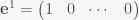
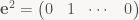
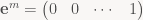
All that said, let’s take another look at matrices. As I explained before (in part 1), the columns of a matrix contain the images of the basis vectors. Let’s give those vectors names:

.

This is just taking the n column vectors making up A and giving them distinct names. This is useful when you look at a matrix product:

.

You can prove this algebraically by expanding out the matrix product and doing a bunch of index manipulation, but I’d advise against it: don’t expand out into scalars unless you have exhausted every other avenue of attack – it’s tedious and extremely error-prone. You can also prove this by exploiting the correspondence between linear transforms and matrices. This is elegant, very short and makes for a nice exercise, so I won’t spoil it. But there’s another way to prove it algebraically, without expanding it out into scalars, that’s more in line with the spirit of this series: getting comfortable with manipulating matrix expressions.

The key is writing the as the result of a matrix expression. Now, as explained before, the i-th column of a matrix contains the image of the i-th basis vector. Since we’re using the canonical basis, our basis vectors are simply


…

and it’s easy to verify that (this one you’ll have to expand out if you want to prove it purely algebraically, but since the product is just with ones and zeros, it’s really easy to check). So multiplying from the right by one of the gives us the i-th column of a, and conversely, if we have all n column vectors, we can piece together the full matrix by gluing them together in the right order. So let’s look at our matrix product again: we wan’t the i-th column of the matrix product , so we look at

exactly as claimed. As always, there’s a corresponding construction using row vectors. Using the dual basis of linear functionals (note no transpose this time!)


…

we can disassemble a matrix into its rows:

and since , we can write matrix products in terms of what happens to the row vectors too (though this time, we’re expanding in terms of the row vectors of the first not second factor):

.

Gluing it back together

Above, the trick was to write the “slicing” step as a matrix product with one of the basis vectors – and so forth. We’ll soon need to deal with the gluing step too, so let’s work out how to write that as a matrix expression too so we can manipulate it easily.

Let’s say we have a m×2 matrix A that we’ve split into two column vectors , . What’s the matrix expression that puts A back together from those columns again? So far we’ve expressed that as a concatenation; but to be able to manipulate it nicely, we want it to be a linear expression (same as everything else we’re dealing with). So it’s gotta be a sum: one term for and one for . Well, the sum is supposed to be , which is a m×2 matrix, so the summands all have to be m×2 matrices too. The are column vectors (m×1 matrices), so for the result to be a m×2 matrix, we have to multiply from the right with a 1×2 matrix. From there, it’s fairly easy to see that the expression that re-assembles from its column vectors is simply:

.

Note that the terms have the form column vector × row vector – this is the general form of the vector outer product (or dyadic product) that we first saw in the previous part. If A has more than two columns, this generalizes in the obvious way.

So what happens if we disassemble a matrix only to re-assemble it again? Really, this should be a complete no-op. Let’s check:

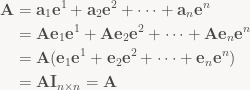
For the last step, note that the summands are matrices that are all-zero, except for a single one in row i, column i. Adding all these together produces a matrix that’s zero everywhere except on the diagonal, where it’s all ones – in short, the n×n identity matrix. So yes, disassembling and re-assembling a matrix is indeed a no-op. Who would’ve guessed.

Again, the same thing can be done for the rows; instead of multiplying by from the right, you end up multiplying by from the left, but same difference. So that covers slicing a matrix into its constituent vectors (of either the row or column kind) and putting it back together. Things get a bit more interesting (and a lot more useful) when we allow more general submatrices.

Block matrices

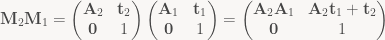
In our first example above, we sliced A into n separate column vectors. But what if we just slice it into just two parts, a left “half” and a right “half” (the sizes need not be the same), both of which are general matrices? Let’s try:

For the same reasons as with column vectors, multiplying a second matrix B from the left just ends up acting on the halves separately:

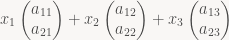
and the same also works with right multiplication on vertically stacked matrices. Easy, but not very interesting yet – we’re effectively just keeping some columns (rows) glued together through the whole process. It gets more interesting when you start slicing in the horizontal and vertical directions simultaneously, though:

Note that for the stuff I’m describing here to work, the “cuts” between blocks need to be uniform across the whole matrix – that is, all matrices in a block column need to have the same width, and all matrices in a block row need to have the same height. So in our case, let’s say is a p×q matrix. Then must be a p×(n-q) matrix (the heights have to agree and is n columns wide), is (m-p)×q, and is (m-p)×(n-q).

Adding block matrices is totally straightforward – it’s all element-wise anyway. Multiplying block matrices is more interesting. For regular matrix multiplication , we require that B has as many columns as A has rows; for block matrix multiplication, we’ll also require that B has as many block columns as A has block rows, and that all of the individual block sizes are compatible as well. Given all that, how does block matrix multiplication work? Originally I meant to give a proof here, but frankly it’s all notation and not very enlightening, so let’s skip straight to the punchline:

Block matrix multiplication works just like regular matrix multiplication: you compute the “dot product” between rows of B and columns of A. This is all independent of the sizes too – I show it here with a matrix of 1×2 blocks and a matrix of 2×2 blocks because that’s the smallest interesting example, but you can have arbitrarily many blocks involved.

So what does this mean? Two things: First, most big matrices that occur in practice have a natural block structure, and the above property means that for most matrix operations, we can treat the blocks as if they were scalars in a much smaller matrix. Even if you don’t deal with big matrices, working at block granularity is often a lot more convenient. Second, it means that big matrix products can be naturally expressed in terms of several smaller ones. Even when dealing with big matrices, you can just chop them up into smaller blocks that nicely fit in your cache, or your main memory if the matrices are truly huge.

All that said, the main advantage of block matrices as I see it are just that they add a nice, in-between level of granularity: dealing with the individual scalars making up a matrix is unwieldy and error-prone, but sometimes (particularly when you’re interested in some structure within the matrix) operating on the whole matrix at once is too coarse-grained.

Example: affine transforms in homogeneous coordinates

To show what I mean, let’s end with a familiar example, at least for graphics/game programmers: matrices representing affine transforms when using homogeneous coordinates. The matrices in question look like this:

where is an arbitrary square matrix and is a translation vector (note the 0 in the bottom row is printed in bold and means a 0 row vector, not a scalar 0!). So how does the product of two such matrices look? Well, this has obvious block structure, so we can use a block matrix product without breaking A up any further:

Note this works in any dimension – I just required that A was square, I never specified what the actual size was. This is a fairly simple example, but it’s a common case and handy to know.

And that should be enough for this post. Next time, I plan to first review some basic identities (and their block matrix analogues) then start talking about matrix decompositions. Until then!

Linear Algebra Toolbox 2

In the previous part I covered a bunch of basics. Now let’s continue with stuff that’s a bit more fun. Small disclaimer: In this series, I’ll be mostly talking about finite-dimensional, real vector spaces, and even more specifically for some n. So assume that’s the setting unless explicitly stated otherwise; I don’t want to bog the text down with too many technicalities.

(Almost) every product can be written as a matrix product

In general, most of the functions we call “products” share some common properties: they’re examples of “bilinear maps”, that is vector-valued functions of two vector-valued arguments which are linear in both of them. The latter means that if you hold either of the two arguments constant, the function behaves like a linear function of the other argument. Now we know that any linear function can be written as a matrix product for some matrix M, provided we’re willing to choose a basis.

Okay, now take one such product-like operation between vector spaces, let’s call it . What the above sentence means is that for any , there is a corresponding matrix such that (and also a such that , but let’s ignore that for a minute). Furthermore, since a product is linear in both arguments, itself (respectively ) is a linear function of a (respectively b) too.

This is all fairly abstract. Let’s give an example: the standard dot product. The dot product of two vectors a and b is the number . This should be well known. Now let’s say we want to find the matrix for some a. First, we have to figure out the correct dimensions. For fixed a, is a scalar-valued function of two vectors; so the matrix that represents “a-dot” maps a 3-vector to a scalar (1-vector); in other words, it’s a 1×3 matrix. In fact, as you can verify easily, the matrix representing “a-dot” is just “a” written as a row vector – or written as a matrix expression, . For the full dot product expression, we thus get = (because the dot product is symmetric, we can swap the positions of the two arguments). This works for any dimension of the vectors involved, provided they match of course. More importantly, it works the other way round too – a 1-row matrix represents a scalar-valued linear function (more concisely called a “linear functional”), and in case of the finite-dimensional spaces we’re dealing with, all such functions can be written as a dot product with a fixed vector.

The same technique works for any given bilinear map. Especially if you already know a form that works on coordinate vectors, in which case you can instantly write down the matrix (same as in part 1, just check what happens to your basis vectors). To give a second example, take the cross product in three dimensions. The corresponding matrix looks like this:

.

The is standard notation for this construction. Note that in this case, because the cross product is vector-valued, we have a full 3×3 matrix – and not just any matrix: it’s a skew-symmetric matrix, i.e. . I might come back to those later.

So what we have now is a systematic way to write any “product-like” function of a and b as a matrix product (with a matrix depending on one of the two arguments). This might seem like a needless complication, but there’s a purpose to it: being able to write everything in a common notation (namely, as a matrix expression) has two advantages: first, it allows us to manipulate fairly complex expressions using uniform rules (namely, the rules for matrix multiplication), and second, it allows us to go the other way – take a complicated-looked matrix expression and break it down into components that have obvious geometric meaning. And that turns out to be a fairly powerful tool.

Projections and reflections

Let’s take a simple example: assume you have a unit vector , and a second, arbitrary vector . Then, as you hopefully know, the dot product is a scalar representing the length of the projection of x onto v. Take that scalar and multiply it by v again, and you get a vector that represents the component of x that is parallel to v:

.

See what happened there? Since it’s all just matrix multiplication, which is associative (we can place parentheses however we want), we can instantly get the matrix that represents parallel projection onto v. Similarly, we can get the matrix for the corresponding orthogonal component:

.

All it takes is the standard algebra trick of multiplying by 1 (or in this case, an identity matrix); after that, we just use linearity of matrix multiplication. You’re probably more used to exploiting it when working with vectors (stuff like ), but it works in both directions and with arbitrary matrices: and – matrix multiplication is another bilinear map.

Anyway, with the two examples above, we get a third one for free: We’ve just separated into two components, . If we keep the orthogonal part but flip the parallel component, we get a reflection about the plane through the origin with normal . This is just , which is again linear in x, and we can get the matrix for the whole by subtracting the two other matrices:

.

None of this is particularly fancy (and most of it you should know already), so why am I going through this? Two reasons. First off, it’s worth knowing, since all three special types of matrices tend to show up in a lot of different places. And second, they give good examples for transforms that are constructed by adding something to (or subtracting from) the identity map; these tend to show up in all kinds of places. In the general case, it’s hard to mentally visualize what the sum (or difference) of two transforms does, but orthogonal complements and reflections come with a nice geometric interpretation.

I’ll end this part here. See you next time!

(Linear) Algebra Toolbox 1

I’m prone to ranting about people making their lives more complicated than necessary with regards to math. Which I’ve been doing quite often lately. So rather than just pointing fingers and shouting “you’re doing it wrong!”, I thought it would be a good idea to write a post about what I consider good practice when dealing with problems in linear algebra and (analytic) geometry. This is basically just a collection of short articles. I have enough material to fill several posts; I’m just gonna write more whenever I feel like it. (Don’t worry, I didn’t abandon my series on Debris, we just had a few gorgeous weekends in a row, and living as I do in the Pacific Northwest sunny weekend days are a limited resource, so I didn’t do a lot of writing lately).

Get comfortable manipulating matrix expressions

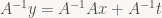
In high school algebra, you learn how to deal with problems such as solving for x using algebraic manipulations. The exact same thing can be done with expressions involving vectors and matrices, albeit with slightly more restrictive rules. It’s worthwhile to get familiar (and comfortable) with this. The most important rules to keep in mind are:

• Vector and matrix addition/subtraction can be handled exactly the same way as their scalar counterparts.
• Since for matrices in general , multiplying an equation by a matrix must be done consistently – either from the left on both sides, or from the right on both sides.
• As an exception to the above, multiplying a matrix/vector etc. by a scalar is commutative, so the direction doesn’t matter, and the scalar can be moved around in the expression to wherever it is convenient.
• Multiplying any scalar equation by 0 turns it into “0 = 0” which is true but useless. For matrix equations, the equivalent is that the matrices you multiply by must be non-singular, i.e. they must be square and have non-zero determinant.

Example: Consider the map . This is an affine transformation, i.e. a linear transformation followed by a translation. Let’s solve this for x: ⇔ ⇔ ⇔ . The only interesting step here is multiplying from the left by , the rest is very basic (and shown in more detail than I will use for the rest of this post). Note the result is in the same form as the expression we started with – meaning that the inverse of an affine map (when it exists) is again an affine map, not very surprisingly.

Matrices depend on the choice of basis

This one is really important.

In linear algebra, the primary objects we deal with are vectors and linear transforms – that is, functions that map vectors to other vectors and are linear. Neither concept involves coordinates. Particularly among programmers, there’s this meme that “vector” is basically just fancy math-speak for an array of numbers. This is wrong. A vector is a mathematical object, just like the number ten. The number ten can be represented in lots of different ways: as text, as “10” in decimal notation, as “1010” in binary notation, as “X” using roman numerals and so forth. These representations are good for different things: decimal and binary have reasonably simple algorithms for addition, subtraction, multiplication and division. Roman numerals are reasonably easy to add and subtract but considerably trickier to multiply, and the textual representation is related to the pronunciation of numbers when we read them out loud, but completely useless to do arithmetic on.

Writing a vector as tuple of numbers is a particular representation that means “one times the first basis vector, plus two times the second basis vector, plus three times the third basis vector”. This representation depends on the choice of basis vectors. Any non-zero vector can end up represented as , given the right choice of basis. Similarly, a matrix depends on the basis for the source and destination vector spaces, and a given linear transform can have any number of different representations, corresponding to different choices of basis vectors. The important bit here is that even though the numbers can be made almost anything, they’re still describing the same mathematical object, and everything that’s true for this mathematical object will be true no matter which representation we pick.

This means that we have a considerable amount of freedom in choosing a convenient representation. As long as we’re writing code that performs computation, we’ll still drop down to matrices and numbers eventually. But generally, we want to postpone that choice until we absolutely have to – the later we nail it down, the more information we have to make the resulting computation easier. And a lot of stuff can be done without ever choosing an explicit basis or coordinate system at all.

What’s in a matrix?

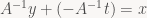
Now I’ve explained what the values in the coordinate representation of a vector mean, but I haven’t yet done the same for the values in a matrix. Time to fix this. Note that with a matrix, there’s generally two vector spaces (and hence two bases) involved, so we have to be careful about which is which. Here’s a simple matrix-vector product expanded out using the usual matrix multiplication rule and then rearranged slightly:

= = .

This is straightforward algebra, but it’s key to figuring out what’s matrices actually mean. Note that the vectors appearing in that last expression are just the first, second and third columns of our matrix A, respectively. Those are vectors in the “output” vector space, which is 2-dimensional here; there’s also a 3-dimensional “input” vector space that x lives in. Often the two spaces are the same and use the same basis, but that is not a requirement! Anyway, if we plug in (corresponding to the first basis vector in our input vector space), the result will just be the first column of A. Similarly, we’ll get the second and third columns of A if we choose different “test vectors” with the one in a different place.

And this is the connection between matrices and the linear transforms they represent: to form a matrix, just transform the i-th vector of your “input” basis and write the resulting vector represented in your “output” basis into column i. This also means that it’s trivial to write down the matrix for a linear transform if you know what that transform does to your basis vectors. Note that here and elsewhere, if you use row vectors instead of column vectors, you write xA, and the role of rows and columns are reversed.

Change of basis

Now to give an example for why these distinctions matter, let’s look at a concrete problem: suppose you have a 3D character model authored in a tool that uses a right-handed coordinate system with +x pointing to the right, +y pointing up, and +z pointing out of the screen, and you want to load it in a game that has a left-handed coordinate system with +x pointing right, +y pointing up (same as before) and +z pointing into the screen. Let’s also say that character comes (as character models tend to do) complete with a skeleton and transform hierarchy. Assume for simplicity that the transforms are all linear and represented by 3×3 matrices. In reality they’ll be at least affine and probably be represented either as homogeneous 4×4 matrices or using some combination of 3×3 rotation matrices or unit quaternions, translation vectors and scale factors, but that doesn’t change anything substantial here.

So what do we have to do to convert everything from the modeler’s coordinate system to our coordinate system? It’s just a few sign flips, right? How hard can it be? Turns out, harder than it looks. While it’s easy enough to convert vertex data, matrices present more of a challenge, and randomly flipping signs won’t get you anywhere – and even if you luck out eventually, you still won’t know why it works now (you can ask anyone who’s ever tried this).

Instead, let’s approach this systematically. Imagine the model you’re trying to load in 3D space. What we want to do is leave the model and transforms exactly as they are, but express them in a different basis (coordinate system). It’s important to get this right. We’re going to be modifying the matrices and coordinates, true, but we’re not actually changing the model itself. Computationally, “express this vector in a different basis that has the z axis pointing in the opposite direction”, “reflect this vector about the z=0 plane” and “flip the sign of the z coordinate” are all equivalent, but they correspond to different conceptual approaches. When you perform a change in basis, it’s clear what has to happen with matrices representing transforms (namely, they have to change transforms to). A reflection is a transform – you might want to apply it to the whole model (at which point it’s best expressed as another matrix you pre-multiply to your transform hierarchy), you might want to reflect part of it, or you might want to just reflect some vertices. All of these actually modify the model (not just your representation of it), and it’s not clear which one is the “right” one. And so forth.

Anyway, enough of philosophy, back to the subject at hand: We have two different bases for the same 3D space: the one used by the modeler (let’s call it basis M) and the one used by your game (basis G). We want to leave the model unchanged and change basis from M to G. The linear transform that leaves everything unchanged is the identity transform I that sends every vector to itself. As mentioned above, every matrix depends on not only the linear transform it represents, but also the basis chosen for the input and output vector space. Let’s make that explicit by adding them as subscripts. We can then write down a matrix that takes a vector expressed in basis M, applies the identity transform (=leaves everything unchanged), then expresses the result in basis G. In our case, the x and y basis vectors in both G and M are the same, while the a vector expressed as in basis M corresponds to in basis G (and vice versa). Putting it all together, we can write down the change-of-basis matrix to G from M:

.

If we wanted to go the opposite way (to M from G), we would use . Now what can we do with this? Well, first of, we can use it to convert vectors expressed in M to vectors expressed in G:

Who would’ve thought, we end up sign-flipping the z coordinate. Written like this, it just seems like a verbose (and inefficient) way to write down what we already know. But note that the subscript notation allows us to see at a glance which basis we’re currently in. More importantly, we can see when we’re trying to chain together transforms that work in different bases. This comes in handy when dealing with trickier objects, such as matrices: note that the transforms stored in the file will both accept and produce vectors expressed in basis M; by our convention, we’d write this as . Now say we want to get the corresponding transform in basis G – well, we could try the same thing that worked for vectors and just multiply the right form of the identity transform from the left:

Oops – see what happened there? That gives us a matrix that produces vectors expressed in basis G, but still expects vectors expressed in basis M as input. To get the true representation of T in basis G, we need to throw in another change of basis at the input end:

So to convert everything to basis G, we need multiply all the vectors with on the left, and multiply all matrices with from the left and from the right (the resulting double sign-flip “from both sides” is the bit that’s really hard to stumble upon if you approach the whole issue in “let’s just keep flipping signs until it works” mode). Alternatively, we can leave all the vectors and transforms as they are, happily working in basis M, but then throw in a single at the top of the transform hierarchy of the model, so that all of it gets transformed into the “game” basis before the rest of the rendering / physics / whatever code gets to see it. Either way works. And not only that, I hope that by now it’s clear why they work.

Note: By the way, this convention of explicitly writing down the source and destination coordinate systems for every single matrix is good practice in all code that deals with multiple coordinate systems. Names like “world matrix” or “view matrix” only tell half the story. A while back I got into the habit of always writing both coordinate systems explicitly: world_from_model, view_from_world and so forth. It’s a bit more typing, but again, it makes it clear which coordinate system you’re in, what can be safely multiplied by what, and where inverses are necessary. It’s clear what view_from_world * world_from_model gives – namely, view_from_model. More importantly, it’s also clear that world_from_model * view_from_world doesn’t result in anything useful. This stuff prevents bugs – the nasty kind where you keep staring at code for 30 minutes and say to yourself “well, it looks right to me”, too.

Implement your solution, not your derivation

This ties in with one of my older rants. This is not a general rule you should always follow, but it’s definitely the right thing to do for performance-sensitive code.

In the example above, note how I wrote all transforms involved as matrices. This is the right thing to do in deriving your solution, because it results in expressions that are easy to write down and manipulate. But once you have the solution, it’s time to look at the results and figure out how to implement them efficiently (provided that you’re dealing with performance-sensitive code that is). So if, for some perverse reason, you’re really bottlenecked by the performance of your change-of-basis code, a good first step would be to not do a full matrix-vector multiply – in the case above, you’d just sign-flip the z component of vectors, and similarly work out once on paper what has to happen to the entries of T during the change of basis.

I’ll give more (and more interesting) examples in upcoming posts, but for now, I think this is enough material in a single batch.

GenThree Overview

This post is part of the series “Debris: Opening the box“.

Now that the code is released, I’m going to change things up a bit. Originally, I was going to describe Werkkzeug 3’s operator execution engine in isolation; but now there’s enough material to give you the story in the proper order, with all the false starts and backtracking that went into it, which should explain some of the design quirks of the final result. Because it all starts with GenThree, the tool we wrote for Candytron (Note: I originally wrote this text for the fr_public repository).

Introduction

GenThree was the next tool Chaos started after Werkkzeug1. See diary.txt for the early history (if you can read German). I joined the project some time after the last entry in diary.txt, in early January 2003. This marks the first time that Chaos and me collaborated directly; before then, Chaos had used my packers, but we hadn’t shared much code.

After joining, I initially took over the Mesh generator and started work on the “FX Chain” (postprocessing effects), while Chaos focused on the GUI and Scripting parts of the system. After the first 2 months or so it rapidly becomes very hard to say who did exactly what because there was no clear top-level division of labor; we worked quite well together, to the point where we sometimes weren’t certain who had written what. As an aside, if you can read German, concept.txt contains a bunch of notes by Chaos, again mostly from the early phases of the project. Some of these ideas ended up in GenThree (and later Werkkzeug3), some never got implemented, and some we tried but rejected.

Scripting

Anyway; even when I started (this was in the lead-up to Candytron), we were very clearly aiming at producing kkrieger; Candytron was intended to be a kind of milestone. The thing that differentiates GenThree from our previous systems was that it was intended to replace the Operator Graph that had been at the center of our previous tools with a scripting language. The Operator Stacking UI still exists, but outputs script code instead of a blob describing the graph. The intention was to use this UI to build up components, but do all of the high-level glue (and, ideally, a lot of the game logic for kkrieger) as a script.

We were considering several kinds of approaches, and different levels of abstraction – e.g. the top of concept.txt has a detailed sketch of a quite low-level scripting system top that would compile to regular x86 code, plus the associated back-end. This was never implemented; the idea evolved into another scripting system that was intended to run-time compile to regular x86 code. Then we’d store the (compressed) byte code plus a small runtime engine instead of regular x86 code, with the hope that the byte code would be smaller. The language was designed to facilitate easy compilation; it was very FORTH-like, so an initial interpreter could just use explicit stacks and threaded code. This one never happened either, primarily because we dreaded going all-in on something this experimental with a code base that was intended to last till kkrieger at the very least. However, the underlying idea (store all our code in a form that’s more amenable to compression) never went away, and some years later metamorphosed into dispack/disfilter, the x86 code transform used by kkrunchy.

But back to GenThree. Scripting system approach number three, and what you see here, was CSL – Chaos’ Scripting Language (he did all the work on that one). The initial idea is described in concept.txt under “Scripted Demo System”. The runtime system is still very FORTH-like, but it uses three stacks instead of the customary two:

• The I-Stack or integer stack, which contains 16.16 fixed point numbers (there’s no support for floating-point types in script code)
• The R-Stack or return stack, used to implement calls, loops etc.
• The O-stack or object stack, which holds references to complex composite objects like Bitmaps, Meshes and so forth. These objects are typed.

The operation of the I- and R-stacks is only visible to the bytecode interpreter; the language itself is C-like and exposes familiar control structures to the user. The O-stack is different; it’s explicitly manipulated by the code.

Rather than explaining this to you in boring detail, I just recommend you check out system.txt. This defines the set of operators available to every project, and displays some of the unconventional features of the system:

At the beginning, a bunch of classes are defined. These correspond to classes of values on the O-stack. The fields listed define instance variables; I don’t remember how exactly that particular binding worked. Each class also has a magic ID, written as hexadecimal number. Since we use 16.16 fixed point, they’re written in a somewhat funky way here; they’re regular 32-bit ints on the C++ side.

After that, there are some global functions and variables. Note that functions can be assigned IDs, just like classes. This is part of a light-weight binding scheme. By convention, positive IDs are used for script functions that are called by C++ code (so the OnInit, OnFrame and OnSound functions are forward declarations for code that’s supposed to be written in CSL), while negative IDs are script declarations for functions implemented in native C++ code. There’s a table in the C++ code mapping those magic numbers to function pointers – and nothing else. Note that each function has type information on the parameters; this is detailed enough to manually build a stack frame and call into the given C++ function, without needing any layer of glue code or marshalling. This is one of the more unconventional design decisions in CSL; it was done both for convenience and to reduce code size, since mechanical wrapper/glue code is very repetitive and adds zero value. Also note that each function comes with a description of what types of objects are expected to be at the top of the O-stack before execution, and what ends up on the O-stack afterwards. To pick a declaration at random:

void MeshMaterial(
  int id = 1 [ 1 .. 255 ],
  int mask = 0 [ "mask8:f" ],
) ( mesh material -- mesh ) = -0x0b,"mod link2",'m';

the ( mesh material -- mesh ) line here denotes that this operator expects a mesh and a material object on the O-stack, and returns a new mesh object. It also means that the op has binding number -0xb (-11), the "mod link2" is a list of annotation tags that can influence GUI, code generation and memory allocation (“mod” here means that the operator can modify an object in-place, for example), and the ‘m’ assigns the hotkey ‘m’ to this operator in the GUI. You get the idea.

There’s even some operators completely written in CSL – cf. the Crashzoom and FXWideBlur filters, both of which make use of the language and call to a single underlying function Blend4x written in C++ that is used to implement various render-to-texture effects.

Going back up a level, I mentioned that there’s still a GUI behind all this. Well, the op-stacking UI is alive and kicking in GenThree, so how does that part work internally? Just look at data/candytron_final_064.csl, the final generated source code for Candytron. The first part of this is just system.txt, which I have just described. After that comes a bunch of generated code corresponding to whatever the user built in the Op-Stacking GUI (this is OnGenerate and friends) and the animation/timeline timeline_OnInit and timeline_OnFrame). All of this is code with a very regular structure that’s intended to compress well. Finally, at the very end there’s the bit starting with // new text – this is actually code entered in the tool itself by the user. The idea was that you could code in there too, but it never saw serious use.

So all this looks pretty nice on paper, right? C++ code providing low-level functions and runtime services, a script engine to tie it all together, and a very decoupled UI that’s loosely coupled: anything that can compile to CSL goes.

The only problem was that (language quirks like the fixed-point centric world view aside) it didn’t work well for what we needed it for. It had reasonable density for code, but as a data representation (and all the Ops are really more data than code) it sucked. Our previous systems had a very compact representation for ops, and lots of tricks to quantize and pack parameter values into a small space. In the byte code-based system, it all boiled down into general “push value” and “call function” op codes, and while the type information was there for execution purposes (to convert the 16.16 ints into floats when necessary, for example), none of that structure was evident or easily exploitable in the byte code. As a result, compression ratios of the byte code sucked – compared to what we were used to, anyway. Candytron had significantly less procedurally generated content than our average intro, yet still spent about 8k (after compression!) on describing it, whereas most of our intros around that time needed maybe 6k for the ops.

On the other side, the script runtime system was fairly big too – much bigger than the more specialized operator execution engines we’d used before (or after). And it just wasn’t pulling its weight. So the summer after we released Candytron, Chaos threw away the scripting parts and most of the existing GUI, but kept the Operators – Werkkzeug3 was born. Still, the base system and most of the content generation parts (and their interface) survived. As one of several side effects, that means that Wz3 used (and still uses) the same “explicit description of stack layout” method for parameters. This has far less benefits in a non-script environment (and we probably wouldn’t have done it if we had been shooting for ops from the beginning), but it’s really just the only part of the original scripting engine that survived.

Code organization

Let’s start at the beginning: _start.cpp (and _startdx.cpp). These two files (plus associated header files) form the OS/rendering abstraction. Yes that’s right, no other file in the project includes any of the Windows or D3D header files, it’s all abstracted away. Fundamentally this is not hard because a demo or intro really doesn’t care that much about what OS it’s running on; what it wants is a window, a nice way to switch state and render triangles, a pipe to output sound to and a way to get current timing information (and maybe keypresses). The tools need a bit more on the input side (proper mouse and keyboard input at least) and some file IO, but it’s still a very limited set of functionality.

The tools use the aforementioned two files; intros use _startintro.cpp, which is a size-optimized mash-up of both _start and _startdx. There’s also _startgdi (for GDI-based GUI-only rendering) and _startgl (GL-based), both of which were never properly completed and don’t work, so there’s not much to talk about.

_start performs initialization and then calls sAppHandler. sAppHandler is implemented in the actual main program and is basically an event handler. To give an example of what constitutes events:

• sAPPCODE_CONFIG – display a configuration dialog. (Called before the 3D API is initialized)
• sAPPCODE_INIT – main initialization phase (after 3D API is initialized).
• sAPPCODE_EXIT – similarly, shutdown phase.
• sAPPCODE_KEY – keyboard input.
• sAPPCODE_PAINT – paint a new frame.

There’s a few more, but you get the idea. There’s two main versions of this: the “tool” runtime in main.cpp and the “player” runtime in mainplayer.cpp. The tool version sets up a window and then runs the GUI event loop; the player version does whatever initialization is necessary and then plays back the demo.

The GUI is a regular retained-mode event loop-based affair. Everything is rendered using the 3D API (D3D in our case) though, and re-rendered every frame, which greatly cuts down on updating bugs :). There’s a lot of UI and UI-related code in GenThree, Werkkzeug3 etc., but that kind of code doesn’t make for very exciting exposition, so I’ll just gloss over it here.

The scripting engine that I’ve talked about is split into two files: cslce.cpp, which implements the scanner, parser and bytecode generator, and cslrt.cpp, the bytecode interpreter and runtime system.

CSL is a language suitable for one-pass compilation with semantic processing and code generation interleaved with code generation. It can be processed with a straightforward Recursive Descent parser. This class of languages has a long tradition and leads to simple, fast (but not very smart) compilers without depending on any special parser generator tools. CSL in particular was greatly inspired by LCC and its code as described in the book “A Retargetable C Compiler: Design and Implementation” – a very worthwhile read if you would like to expand your horizon on a type of Software Engineering that’s underappreciated: Simple, straightforward, very well thought-out no-nonsense C code. (As you might be able to tell, Chaos and me really like that book). Anyway.

The second part, cslrt, implements the runtime. Since the bytecode is stack-based with a small set of built-in operations, this is really quite straightforward.

On the player side, the rest of the source, including all the generators, binds loosely to the script runtime, which calls the shots. The table of script functions, together with some glue code, is in genplayer.cpp. The rest is just a bag of script-callable functions, which I’ll describe one functional group at a time.

Mesh generation

This is something we tried to push hard for this intro – much more so than in our previous releases. The mesh generator contains a bunch of ideas, some
of which worked out well, and lots that didn’t. The core mesh data structures are half-edge based, and the implementation is contained in genmesh.cpp and genmesh.hpp. I’ve written about this in detail before – just look at the mesh-processing articles linked from the parent post.

One part I haven’t talked about before, and that only appears in GenThree, is the Recorder – the Rec* group of functions in the GenMesh class. This was an experimental approach for mesh animation that we used heavily in Candytron. The basic idea was to separate the topological processing (which involves tricky and often slow manipulation of complex data structures) from the vertex processing (which, for a lot of operators, simply computs new vertices as linear combinations of existing ones, which is simple and relatively fast).

So Chaos had the idea to separate the two. The topological processing just runs once, at init time. All the topological modifications are done at that time, but vertex manipulations get recorded to a log. Most of the time, this log is played back immediately and then thrown away – but if the user wants to animate something, he can turn on “proper” recording for the mesh, which means that we actually keep the log for runtime evaluation. Then, every frame, a bunch of input parameters can be changed and the log is played back. Since we only modify vertices not indices or connectivity, we just need to stream the new data into a vertex buffer. This system is far more flexible than regular skinning; several scenes in Candytron first skin the girl mesh (unsubdivided), then subdivide it once, extrude parts of it, and subdivide again, for example. The extrusion and subdivision operators are relatively heavyweight, since they try to deal correctly with hard edges, discontinuities and so forth, but the part that runs at runtime only only does very simple operations on vectors, so it’s quite fast.

While a neat idea, we ultimately killed this one off too. It worked just fine, but in practice just phrasing all our dynamic mesh animation in terms of skinning made things simpler and more orthogonal at the back end, allowed us to do more work in the mesh consolidation/vertex buffer generator phase, and simplified the mesh code a bit (since there was no longer a need to separate topology and geometry processing into two parts and explicitly record every parameter that went into vertex generation). And finally, a single static skinning setup can be baked into a vertex shader for performance; the more complex recorder system, with its variable input-output relationships and different operations done in different sequence, not so much. Note that we still ended up using SW skinning in kkrieger/debris for other reasons (shadow volumes), but the decision to remove the recorder was made long before we commited to shadow volumes.

Finally, there’s Mesh_Babe, which was used to get the girl mesh (her name is “Josie”, by the way) into the intro. On the Editor side, this just loads an exported mesh (.XSI file in this case, since giZMo – the artist on this project – was using XSI). However, the XSI file is much too big to use in a 64k, so we implemented some (then) cutting-edge mesh compression; the papers had only been published a few months prior! The algorithm we ended up using was described in “Near-Optimal Connectivity Encoding of 2-Manifold Polygon Meshes” by Khodakovsky et al.; there was a separate paper “Compressing Polygon Mesh Connectivity with Degree Duality Prediction” by Isenburg that described the same basic idea in a slightly different framework that probably would’ve been easier to implement in GenMesh, but I realized that too late. I’ll spare you the details – suffice to say this was my first (but by no means last) contact with the fact that being able to understand a paper and being able to implement it correctly are two different things, and one of them is much harder than the other :).

Anyway, the idea was that we’d generate rough basic geometry for kkrieger using a conventional modeler and export it. That was in fact the main reason to be implementing a polygon mesh compression scheme that was this general. But in the end we went down a very different road for level building, so this code too ended up being unused anywhere else. (Starting to see a pattern here?)

Texture generation

This code has the distinction of being the least experimental of all the things we tried in Candytron. It also is the only piece of the whole thing that survived into the Debris era without being substantially rewritten or outright replaced. Part of this was the Second System Effect (e.g. GenMesh was clearly overengineered for what we needed), but mostly it was just the result of us going out of our comfort zone established in previous tools and trying to approach things differently. Most of the time it didn’t work out that well, but it wasn’t at all obvious from the outset that this would happen, and it was certainly a learning experience.

Anyway, on to the actual texture generator. Like the RG2 texture generator (but unlike the original fr-08 Generator or Werkkzeug1), GenThree uses an integer format with 16 bits per color channel, to make sure there’s enough precision headroom even after several stages of color adjustment and layer composition. Though we store 16 bits per channel, we actually only use 15 bits – a compromise to navigate the odd set of MMX instructions available at the time: note that PMULHUW was only added with the Pentium 3, and there’s no unsigned version of PMADDWD – dealing with unsigned 16-bit quantities was simply awkward. We also allow ourselves to be slightly sloppy with regards to rounding and such, since we have enough extra bits not to care too deeply about what goes on in the least-significant bits. This makes the code somewhat simpler, though in the grand scheme of things, it probably didn’t matter. Finally, this representation means that a single ARGB pixel fits inside a MMX register, and there’s no need to do any unpacking or packing to do multiplies (MMX only provides 16-bit multiplies).

As you might have noticed by now, all of these decisions were made with an eye towards reasonably fast and simple implementations of the basic operations using MMX. It was all designed long before using GPUs for texture generation was a serious option: when GenThree was written, we were already using D3D9 (brand new at the time!), but we were using the fixed-function pipe – cards with shader support were still quite new and not very wide-spread. And when RG2 (which made many of these original design decisions) was written, there wasn’t any programmable HW in the PC market, period.

So you would expect that there’s lots of MMX code in the texture generator. And you would be completely right. At the time, code generation when using intrinsics was simply dreadful, so it’s mostly inline assembly too. The code itself is not terribly interesting – it does what you’d expect, and this was from before we did any tricky optimizations. It’s probably worth looking at the Blur filter, however; it uses the old (as in, OLD) but still awesome rendering trick of factoring triangle filters and gaussian blurs as iterated box filters: 2x box gives you triangle, and 3x box gives you a uniform B-Spline that is within a few percent of a true Gaussian but much cheaper to compute. The nice bit about this is that box filters are really simple to do fast – for every pixel, you scroll the “window” by one pixel, meaning one pixel on the left “drops out” and one pixel on the right “comes in”, while the rest of the sum stays the same. This is very cheap to perform incrementally, and Bitmap_Blur has a straightforward implementation of the idea. Look closely – by the time you’ll see it next in this repository, namely in Werkkzeug3, it will support non-integer blur kernel widths and be all MMX’ed up and quite hard to follow :) (It’s the subject of its own upcoming blog post; go figure).

Lights, Camera, Action!

Lighting, material, camera and scene description all happen in the same file, genmaterial.cpp. All of these are objects, so they have a description as a data structure, but in GenThree these are quite basic. A scene is a list of meshes with associated transform matrices. A camera is just a matrix with a few extra parameters describing FOV and such. A light is also just a bag of values that gets passed along to D3D. A material both contains D3D “material” parameters (which influence lighting) and the textures and render states used at the time. States are generally collected once at initialization time and compiled into a list (for faster state caching), but other than that it’s pretty simple too. The most important part here is that an explicit material representation that describes *all* the state sent to the API is even there. In a heavily data-driven environment like our tools, that is just the natural way to handle things; that it also happens to be efficient is a nice bonus.

The most interesting part of genmaterial has in fact nothing to do with materials at all; for reasons that I don’t remember, part of the GenMesh implementation is in here, namely the part that actually converts GenMeshes to Vertex/Index buffers. Sometime in the middle of kkrieger development, all of the mesh preparation, lighting/material and multipass management stuff got pulled out into a separate module, engine.cpp, where it’s resided ever since. Of course, when we wrote Candytron, all of this code was much simpler, so there you go.

There’s two interesting bits worth noting here: first, note how we handle vertex/index buffers. GenThree introduced GeoBuffers, which bundle a Vertex Buffer with an associated Index Buffer into a neat little package. This model (in one form or another) has been around with us ever since – you really want to treat them as a unit most of the time. The system level code (in _startdx.cpp) handles all the memory management part of it – pretty sweet. There’s also a special GeoBuffer that has a static index buffer (describing a list of quads) that’s used to render, well, quads. For GUI, particles and such. It makes sense to have this as part of your rendering abstraction; quads are common, and having a simple way to render them just makes sense. Also, if you make them a thing at the system level, it’s trivial to adapt to targets that natively support non-indexed quad lists.

The second part is that the mesh preparation code supports several different modes (or “programs”, as they’re called in the code): There’s MPP_STATIC and MPP_DYNAMIC, which are fairly obvious (allocate to dynamic/static vertex buffer please); more interestingly, there are also the “sprites”, “trees”, “thick lines”, “outlines”, and “finns” modes, which are also extensively used in Candytron. All of these represent different ways to turn a given mesh into a vertex and index buffer. The same mechanism was used in kkrieger to generate input data for shadow volume extrusion (note that while there is a MPP_SHADOW there, that’s a different thing than what we did in kkrieger).

That’s all, folks!

There’s more stuff in there, but this covers what I think are the most interesting bits. If there’s questions or something is unclear, don’t hesitate, just ask!

If in doubt, go to the source

This post is part of the series “Debris: Opening the box“.

As mentioned in the introduction to this series, our various demo tools contain a lot of cool ideas, but also a lot of bad ones that didn’t work out, and the code has suffered as a result. Nevertheless, the code makes for an interesting historical document if nothing else, and we (Farbrausch), after some deliberation, decided to just open it up – something we’ve been planning to do for ages, but were never able to pull of for various legal reasons. Well, all of those problems have gone away over the past year, so there was no good reason left to not publish the source.

So here it is: https://github.com/farbrausch/fr_public.

We decided to go with very permissive licenses: a lot of the code was released into the public domain, the rest is BSD-licensed, and all of the (currently uploaded) content is released under Creative Commons CC-BY or CC-BY-SA licenses. So if you want to play around with it, go ahead! Also, we will be adding both more demos and code as soon as we’re able – re-licensing these things means we need to acquire permission from all the original authors, which takes a few days to sort out. Similarly, some of the code we’re planning to release contains optional components encumbered with third-party rights that we need to get rid of before we can make it public.

Finally, there’s some ongoing “reconstruction” work, too: the original code was written for various compiler versions etc., and some depended on old library versions that are no longer available. A separate branch of the repository (“vs2010”) contains modified versions of the original code that should compile with VS2010.

And what about this series? Don’t worry, the point I made in the first post of this series remains valid: Source code is a good way of communicating cookbook recipes, but a bad way of describing the underlying ideas. So this series will continue, only from now on, you’ll be able to cross-check against the actual source code and notice all the little white lies I’m telling to make things easier to follow or understand :)

UPDATE: Turns out Memon just decided to release source code for Demopaja, his demo-tool, too! The more the merrier.

Metaprogramming for madmen

This post is part of the series “Debris: Opening the box“.

Okay, previous posts from this series aimed to actually convey useful technical information: assuming you actually want to write say a mesh generator, there’s definitely useful bits there.

This is not one of these posts. In fact, this is about what is pretty much the complete opposite: an insane ploy that, against all odds, actually kinda worked, then spectacularly backfired. We knew ahead of time this was gonna happen, but we were desperate. I don’t think there’s anything of any use we actually learned from the whole thing – but it makes for a cool story (in a very nerdy way), so why not? Consider it a (seasonally appropriate!) easter egg.

The setting

This is recounting a true story that took place in late March and early April 2004 – a bit less than 2 weeks before Breakpoint 2004, where we planned to release our 96k first-person shooter “.kkrieger”. While being a nice technical challenge, it was a complete failure as far as the game side was concerned (mostly because no-one involved really deeply cared about that aspect). That’s not what this post is about though – the point is that we very nearly missed the 96k limit too.

The way any self-respecting 4k intro, 64k intro or other size-limited program starts out is, well, too large. I haven’t done enough 4ks to give you an order of magnitude estimate, but most of our serious 64ks were somewhere around 70-80k a few weeks before they were supposed to be released. The last 2 weeks usually ended up turning into a frenetic rush to simultaneously get the thing actually finished (put all the content in etc.) and make it fit within the size limit. Doing either of those is a real challenge by itself. Doing both at once is both extremely stressful and mentally exhausting, and by the end of it, you’re basically in need of a vacation.

Anyway, there’s (broadly speaking) 3 different steps to making sure you get small code:

1. Architecture. Basically, design the code in a way that enables it to be small. Know exactly what goes into it, keep it modular, and make sure the algorithms are appropriate. Store data in the right way, and work with your back-end packer, not against it. All of this is pretty much over 2 weeks before release though – if you didn’t get that part right early enough, you’re not gonna be able to fix it in time.
2. Evicting ballast. There’s gonna be whole paths of code that are just not getting used. If your data doesn’t have a single torus in it, there’s no point including the code that generates it – and if there’s just one torus, you can maybe replace it with something else in the art. You get the idea. This step is fairly easy provided you have at least rudimentary stats on your content, and it yields big wins in short time (in a 64k context, usually several kilobytes for less than an hour of work).
3. Detail work. This is where it gets messy. It basically boils down to dumping stats about all of the functions in the code, figuring out which are larger than they should be and what you can do to make them smaller. Lots of staring at disassembly listings trying to find out where the compiler is generating big code and why. Also lots of time staring at the content and figuring out if there’s some shortcuts you can take to make this particular intro smaller. This is where you start switching to a different branch (or at the very least wrap all of your changes in #ifdef) because you’re going to introduce bugs and by the end of it, parts of the code are gonna be ruined. It’s also slow work – by the point the initial easy targets are down, and assuming there’s nothing else to do, I can get 32-bit x86 code (in a 64k intro context) smaller at a rate of about 300-400 bytes per day, tops.

Basically, by the end of step 2, you have a pretty good idea of how much more work is left, even though you have very little clue of what that work is :). Note this is very different from things like speed optimization. For speed optimization, you’re usually willing to make significant changes to data flow to do less work, at least where it matters, and you concentrate on hot spots. For size optimization, hot spots are mostly irrelevant; sure there may be a place where a big array ends up being initialized by code rather than being stored as data, and fixing that kind of thing is usually easy and fun, but mostly the hot spots in a “size profile” are the places where the actual work gets done. Unless you actually do work that is completely unnecessary, optimizing for speed will not make your code smaller in an absolute sense, it will just move the complexity (and thus size) somewhere else in the executable image.

Speed micro-optimization is about staring at loops and figuring out how to make them tighter. Size micro-optimization is about staring at large bodies of code and figuring out how to either get rid of it completely, share code with something else that’s similar enough, or doing small architecture-specific tricks with an “area effect”. For example, on x86, you can reorder struct fields so the ones you access most often – in terms of distinct instances, not number of times they end up being executed – end up within 127 bytes of the base pointer so 8-bit displacements get used. Things like that.

With that established, let’s get back to kkrieger.

98304

The first time we got the “player” versions of kkrieger running, the compressed executable was something like 120 kilobytes. By the time we had thrown out all the ballast and were finished tweaking the data formats, we were down to about 102k, but that was still with some content (and good chunks of the game – not that there was that much to begin with!) missing. A bit more than two weeks before the release, we started meeting (more or less full-time) at Chaos’s place to put it all together – note things were complicated by the fact that Chaos, me, and giZMo (one of our two artists) were also organizers of Breakpoint, the party where kkrieger was to be released, so we also had to arrive early at the party place, build everything up and so forth. So we knew there was maybe a week and a half left, and the aforementioned frenzy set in – worsened by the fact that a lot of the art was still incomplete (and parts of it were broken in the small “player” executable) and there were gaping holes in the game code (most importantly, some serious collision issues that we never fixed). Lots of work and little sleep. At some point, Chaos put up a (hand-drawn) sign saying just “98304”, the target size (in bytes) we were aiming for – 96 (binary) kilobytes.

A week before release, we were at 100k. The realization started to sink in: At the rate we were going, this was not going to work out – unless we were willing to throw out large amounts of content, which we really didn’t want to. We needed to change gears and come up with another plan, fast.

A plan so insane, it might just work.

The key idea was that, in the “detail work” step, there’s lots of things you could do if you were willing to really specialize the code to the content. As in, literally throw out all code paths that will never be taken for the given content. In the final shipping executable, everything is procedurally generated from the same source data, always; the code in the player needs to work for that one data file and nothing else. There’s a big catch, though: it’s a time sink to manually determine exactly which code paths are actually necessary, and once start going down this road, you really cannot touch the data anymore.

In short, doing this manually is not only crap work, it’s also extremely brittle – which is why we never did this for any our previous 64ks. However, in this case, we were desperate, and we really just didn’t have any other idea of what else we could do to shave off 4 kilobytes in a week. So we did what any self-respecting programmer would do in this situation: we decided to write a program to do it for us.

The idea was this: We decided to write a new tool, “lekktor” (always with the double-ks, I know). It’s a play on the German word “Lektor” which means editor, as in person who edits books, not text editor. Lekktor was to take the program and instrument it with detailed code coverage tracking. Then, in a second pass, it would take the code coverage information gathered in the first pass and eliminate all the paths that were never taken. Since all the content generation is deterministic and happens at the start of the program, you’d just need to launch the game once in instrumented mode, take the dumped coverage information, then run lekktor again to write the “dead-stripped” source files and recompile.

Sounds relatively simple, right? The only problem being that it involves parsing and processing C++ source code.

My kingdom for a pretty-printer

Chaos’ original idea was to start from a source code pretty-printer (think GNU indent and programs like that). Note that the kind of source processing described above doesn’t really care about declarations and types, the two trickiest bits of C++. Really, all you need to know to be able to do this kind of processing is to detect and parse certain kinds of statements and expressions: if, else, for, while, do, and the &&, || and ?: operators. We figured that a source code pretty-printer should understand at least that much about C++ code, and then we could add some extra tokens in strategic places and we’d be set.

Alas, we spent an afternoon looking at different such packages, and none of them actually understood even that much about C/C++ code; they were mostly trying to make do with regular expressions. That wasn’t gonna fly for what we needed. At the end of the day (the Sunday before Easter Sunday, 2004), we hadn’t found anything useful – we had a plan, but no way to make it work.

That’s when Chaos decided that, “well, guess I’ll need to write my own C++ parser then”.

What, you think I was kidding with the title of this post? Note we had about 3 days total to make this work, and we were going all in by doing this; if this hadn’t worked out, we’d have been screwed. Luckily, it did work out. Sort of.

Parsing C++ – how hard can it be?

Turns out, not that hard, provided you a) only need to do it approximately, b) can just change the program you’re trying to parse to work around problems, and c) are willing to take some shortcuts to simplify matters considerably. We didn’t need to be able to parse template declarations, for example; in fact, we just parsed unpreprocessed C++ source files, and skipped on headers entirely (we didn’t have any significant amount of code in headers, so there was no reason to). That meant we needed to modify parts of the code so that #ifdef and the like didn’t mess with the control structure. For example, stuff like

    if (condition)
    {
        // ...
    }
#ifndef IS_INTRO
    else (condition_2)
#else
    else (condition_3)
#endif
    {
        // ...
    }

wasn’t allowed – not a big loss, but you get the idea: we were totally willing to reformat code in fairly simple and mechanical ways if it meant we’d get our code coverage analysis.

The next morning, Chaos had to take a break from his “vacation” time and go to a work meeting in Berlin. That meant a roughly 2-hour train ride in each direction; he took his laptop, a pair of headphones and a copy of “A Retargetable C Compiler: Design and Implementation” with him. By the time he came back in the late afternoon, he had a very rough parser that could “understand” simple functions – and, of course, indent them properly :). By the time we went to sleep that night, we had it working on parts of our target codebase.

By noon the next day, we could process significant chunks of the code we were interested in, and in the early afternoon, we added code coverage tracking and “dead code elimination”. The first worked by assigning unique IDs to each location and just incrementing a corresponding counter whenever execution got through there; the second, by adding if (0) in strategic locations (way easier than actually removing the code yourself – just let the compiler’s dead code elimination deal with it!).

To give an example of what it did: Here’s a short original fragment from GenMesh that deals with selection processing:

void GenMeshElem::SelElem(sU32 mask,sBool state,sInt mode)
{
  switch(mode)
  {
  case MSM_ADD:    if(state) Mask |= mask;                     break;
  case MSM_SUB:    if(state) Mask &= ~mask;                    break;
  case MSM_SET:    if(state) Mask |= mask; else Mask &= ~mask; break;
  case MSM_SETNOT: if(state) Mask &= ~mask; else Mask |= mask; break;
  }
}

and here’s the same code after Lekktor was done with it (run using the kkrieger data):

void GenMeshElem::SelElem(sU32 mask,sBool state,sInt mode)
{
  switch(mode)
  {
    {
    }
    case MSM_ADD:
    {
      if(state)
      {
        Mask|=mask;
      }
    }
    break;
    {
    }
    case MSM_SUB:
    {
      if(state)
      {
      }
      if(1)
      {
        Mask&=~ mask;
      }
    }
    break;
    {
    }
    case MSM_SET:
    {
      if(state)
      {
        Mask|=mask;
      }
      else
      {
        Mask&=~ mask;
      }
    }
    break;
    {
    }
    case MSM_SETNOT:
    {
      if(state)
      {
      }
      if(1)
      {
        Mask&=~ mask;
      }
      else
      {
      }
      if(0)
      {
        if(0)
        {
          Mask|=mask;
        }
      }
    }
    break;
    {
    }
  }
}

Aha – looks like that for this function, the MSM_SUB path only ever gets called with state true, and same for the MSM_SETNOT path, so we can get rid of the ifs. Yeah, that’s the kind of thing you would never ever consider doing manually; it’s obviously extremely brittle and it only saves a handful of bytes (a single compare and a conditional branch). But that’s exactly the point – saving hundreds of bytes in one place can be done well by human optimizers. Saving 3-5 bytes in a thousand places, not so much.

Note that for every if, we keep track of whether it’s either never or always taken; we still need to evaluate the if expression (which might have side effects!), so the original if stays, but we yank everything out of the body and instead put it into a if (0) (or if (1)) block. Again, let the compiler’s data-flow analysis deal with the rest to clean this mess up!

So, after about two days of work, we had something that could, conceivably, make a significant dent in our size profile. So we started ran it on GenMesh and GenBitmap (you can guess what those two things do). And it worked! And saved about 2.5k – more than halfway to our target! That’s when we realized our insane plan might actually work out. Only problem being, we still had 1.5k to go, and we had to leave for Bingen to start with Breakpoint 2004 location set-up the next day.

Fast forward

I’ll spare you the details of the next few days; they add little to this particular story. We did get to save about 4.5k using lekktor in the end, meeting our goal. Of course our ambitions increased a bit too; there was this small intro sequence we had lying around but were willing to get rid of (since it really had nothing to do with the game). Once we were getting close, we kept pushing trying to get to keep the intro too. But it was a tall order – this was essentially the only sequence in the game using cut scene-like functionality, so it was pulling in a lot of code that wasn’t necessary for anything else, and cost a lot more than just the data. And of course there were tons of last-minute content tweaks and (ultimately futile) attempts to clean up the broken gameplay.

By 2 hours before the competition started, we had a version without intro that fit inside the 96k limit, and a version with intro sequence that was 0.5k over the limit. Because we had other stuff to work on over the week, we’d mainly gotten there by (carefully) moving more and more source files over to lekktor. We had a magic #pragma you could use to turn processing on and off for regions of code; slowly we kept pushing deeper and deeper into the whole project. We started “lekktoring” not just the fully deterministic content generation code, but also things like the low-level init code, parts of the 3D engine, and parts of the game code. We tried to be careful to mark up “taboo” sections correctly, but we were operating under severe stress, with tons of other stuff to do at the same time, and with not enough sleep, so we got sloppy in some places.

Suddenly, one and a half hours before the competition (and several hours after the deadline – benefits of being an Organizer…), Chaos came up to me smiling, saying that he’d done some refactorings on the code and re-did a Lekktor run, and now we did in fact have enough space to keep the intro sequence in! Needless to say, we were elated, packed the whole thing up with the README, zipped it and shipped it (so to say).

Of course, at this point you can imagine what had actually happened. So for our shared entertainment value, here’s the full list of things (so far as I know) he didn’t trigger during his trial run, which subsequently got compiled out of the released version:

• We used shadow volumes; there was a shadowing path for one-sided stencil cards (two passes) or two-sided stencil cards (one pass). The card we were recording on (a GeForce4 Ti) had two-sided stencil, so the one-sided stencil code didn’t make it into the released version. Oops. (This one had nothing to do with “user error” during the trial run).
• In the menu at the start, cursor-down works, but cursor-up doesn’t (he never hit cursor-up in menus during the test run).
• The small enemies at the start can hit you, but he didn’t get hit by any enemy shots, so in the released version of .kkrieger enemy shots deal no damage.
• Part of the collision resolution code disappeared, since it was never used in the trial run.

For what it’s worth, this was maybe 230 bytes of code or so. Hey, considering we pretty much removed random ifs, that’s a quite short list actually! :)

So what did we learn?

Honestly? I’m not quite sure. The story has a nice poetic justice to itself though, and I promise that I really didn’t make any of this up – all of this actually happened like I described!

In reality, we knew this was a bad idea when we started, but on the other hand, this was one of the best bad ideas we ever had :), and some mistakes are worth making (once). And both Chaos and me were well aware that we were practically begging for something like the magically lost collision code to happen by doing this kind of stuff. But we were desperate and we really wanted to release kkrieger at Breakpoint, and we did, so it all worked out in the end. kkrieger was a crappy game with or without the bugs mentioned above; at least this way I got a nice story to tell.

Well, that and a running gag. In numerous occasions after .kkrieger, when we were working on intros, and hitting the size-optimization phase, one of us would suggest “well, you know, we could dig up Lekktor again…”. And then we’d both shudder and just shake our heads.

Half-edges redux

This post is part of the series “Debris: Opening the box“.

Here it is, the conclusion to my half-edge based mesh generator miniseries (the data structure part, at least). The first two parts covered the data structures used in GenMesh, the “old” mesh generator. In this part, I’ll be talking about GenMinMesh, the successor to GenMesh which (as they name suggests) was designed to be much more minimal and more suitable for 64ks. As described in the last post, GenMesh tries to build everything out of a small set of primitive operations. The advantage is that the actual data structure manipulation and its associated complexity is concentrated into a few functions. Most of the remaining code defers the data structure management to those few functions; what remains is code to set up and modify vertex positions and attributes – the part that you’ll find in any mesh generator. The problem is that anything that uses the mesh generator at all will end up referencing most of that basic functionality, even if you only ever use (say) one type of primitive. Not a big deal for .kkrieger (which after all used most of the code we had at the time) and Debris (where we didn’t care at the time), but it was an issue for 64ks (not that we seriously pursued any 64k projects after Candytron). Also, GenMesh was fairly slow (mostly because every operation looped over the whole mesh to keep things simple, which meant all the repeated-extrusion stuff hurt on big meshes) and it was painful to deal with operations that resulted in meshes that weren’t necessarily 2-manifold (or had them as temporaries).

Hence GenMinMesh. And to get it out of the way, GenMinMesh is not actually a half-edge based mesh generator. It’s organized around conventional face and vertex structures (slightly more sophisticated than a plain index buffer, but not by much), but knows how to produce half-edge adjacency information for the operations that need it. The data structures are simpler, there’s way less pointer chasing, it’s easy to create a mesh, and there might even be unicorns and rainbows involved! (Not really). So let’s get started.

Back to the basics

We’re going to sacrifice some flexibility and go to a structure with a maximum number of edges per face – allowing us to make the core data structures a lot more straightforward:

static const int KMM_MAXUV = 2;   // max number of UVs per vertex
static const int KMM_MAXBONE = 4; // max bones per vertex
static const int KMM_MAXVERT = 8; // max vertices per face

struct GenMinVert                 // a vertex
{
  bool Select;                    // selected or not
  U8 BoneCount;                   // how many bones in use?
  U16 Temp;                       // mostly padding

  Vec3 Pos;
  Vec3 Normal;
  Vec3 Tangent;
  Vec2 UV[KMM_MAXUV];
  float Weight[KMM_MAXBONE];      // bone weights
  U16 Matrix[KMM_MAXBONE];        // bone matrix index
};

struct GenMinFace                 // a face
{
  bool Select;                    // selected or not
  U8 Count;                       // edge count
  U16 Material;                   // material index, 0=deleted

  Vec3 Normal;                    // face normal
  int Vertices[KMM_MAXVERT];      // vertex indices
  int Opposite[KMM_MAXVERT];      // adjacency - see below
};

Note that this time, the vertices don’t just describe connectivity, they have payload; in fact, they’re almost all payload. GenMesh was designed to support variable vertex formats. As a result, there’s basically no geometric information in the vertex structure – there are separate arrays for positions, normals, UV coordinates etc., all of which might are indexed by the vertex number. If the mesh needs a second UV set, allocate space for that array, otherwise it’s just a null pointer. This was flexible, but we never really ended up using that many different vertex formats, so this time we just opted to go for a fixed fat vertex layout that had everything we might conceivably use. This might still get converted into different vertex formats later down in the pipeline (where it’s easy), but the mesh processing code doesn’t have to be aware of it.

Why a maximum of 8 vertices per face? Well, that number clearly has to be at least 3 (triangles), and since we still want Catmull-Clark subdivision it should really be at least 4 (besides, almost all our primitives are mostly made of quads). What about larger faces? For a planar graph (or any other graph with Euler characteristic 2, which happens to include all meshes isomorphic to a sphere, i.e. connected 2-manifolds without holes) where each vertex has a minimum degree of 3 (i.e. it’s not just made of lines), a well-known fact is that the average face must have less than 6 edges (this can be derived from the Euler formula with some algebra), and it can’t have less than 3. So if we make the limit 6 (or higher), we know that higher-degree faces are going to be rare in any mesh we’re likely to encounter – we could either special-case them or make sure they’re never created in the first place. GenMinMesh opts for the latter, for simplicity (the actual limit is 8 because, well, 6 isn’t a power of 2…).

So where’s the half-edges?

One prominent thing I haven’t mentioned so far is the half-edges. Indeed, what I’ve described so far is a classic face-vertex structure with no edge information at all. Don’t worry, the connectivity information is still there, but it’s a lot more implicit than in the previous two posts.

Remember that a half-edge is a directed edge between two vertices that belongs to a single face. Now, in a face-vertex structure, we store indices of all the vertices belonging to a single face, in order. The half-edges making up a face are implied to be between subsequent vertices in that list. In fact, if we specify both a face and a position in the ordered vertex list, we can uniquely identify any given half-edge: the pair (face, slot) denotes the half-edge from face.Vertices[slot] to face.Vertices[(slot + 1) % face.Count] (indices are taken mod face.Count to handle wrap-around). For convenience, let’s use the fact that we limit our polygons to a maximum of 8 edges to pack that face/slot pair into a single integer: e = face_id*8 + slot (the half-edge ID). Now, let’s have a look at the half-edge diagram from the first part one more time, and check how much of the connectivity information we have covered at this point:

• e itself: Check – we can uniquely reference each half-edge in the mesh.
• start(e): Check – this is just face.Vertices[slot] (and as noted in the first part, we only need to store one of the two vertex indices for each half-edge, so we’re good).
• face(e): Check – since e is just a face/slot pair, we again can recover this one easily.
• next(e): We just need to move over to the next slot in the same face – again, with wrap-around. So next(e) = next((face, slot)) = (face, slot+1 % face.Count).
• prev(e): This time we decrement instead of incrementing, but otherwise it’s the same.
• opposite(e): Aha, this one we don’t have, and there’s no fast (i.e. non-“search everything”) way to recover it from just the face and vertex lists. And there’s this ominous-looking Opposite array in our face structure. The plot thickens.
• (Not pictured) faceEdge(f): For a given face, it’s trivial to name a half-edge that belongs to it: (f, 0) (slot 0 for the given face) should do.

So as you can see, we already have most of the connectivity information we care about; all we need to do is to keep track of the opposite half-edges explicitly, the rest we can just infer from the face-vertex information. As described above, it’s easy to pack a (face, slot) pair into a single integer, which are precisely the integers we store in the Opposite array. Note that, in a sense, this layout is dual to the data structure described in the previous part: there we stored opposite half-edges together but needed explicit links for everything else, here it’s precisely the other way round.

Throw-away connectivity

A problem with the standard half-edge representation is that some basic operations (the most notorious one would probably be adding a single triangle to a mesh) end up being tricky with lots of different cases to consider. The nice thing about the face-vertex structure described above is that faces are still easy to manipulate (in particular, adding new faces is easy). The problem is that operations such as adding a face in the middle of the face list (or a vertex in the middle of a face) will affect multiple edge IDs, effectively breaking existing links.

The way GenMinMesh resolves this (and related) problems is quite simple. Opposite information is not guaranteed to be current; operators might or might not update it. However, there is a single boolean for the whole mesh denoting whether connectivity information is current. All operations that break links clear this flag. Now, if an operation that needs full connectivity (such as mesh extrusion) gets an input mesh that’s not up-to-date, connectivity information gets rebuilt (this boils down to setting all Opposite links correctly).

The assumption is that, when in doubt, the list of faces and the per-face vertex lists are always right. To rebuild connectivity, we first build a list of all half-edges in the mesh in a temporary array. We want to match up opposite pairs; to make this work, we store not just the corresponding half-edge ID but also the IDs of both vertices connected by the half edge, and (arbitrarily) define that the first vertex has to have a lower ID than the second vertex. We then sort the whole list lexicographically by those vertex IDs – any decent sorting algorithm will do. After the sorting process, opposite half-edges will be adjacent in the list, which makes the process of pairing up neighbors straightforward. In pseudocode: (a bit Python-y this time because my usual C-like pseudocode is poorly suited to express data structure iteration concisely)

half_edges = []
for face in (mesh.faces) {
    for e in (face.half_edges) {
        half_edges.add(edge_desc(id=e.id,
                         v0=min(start(e), end(e)),
                         v1=max(start(e), end(e))))
    }
}
half_edges.sort(keys=v0, v1)

for i in (1..len(half_edges)) {
    prev = half_edges[i-1]
    curr = half_edges[i]
    if (curr.v0 == prev.v0 && curr.v1 == prev.v1)
        connect_halfedges(prev.id, curr.id)
}

Regenerating connectivity information is thus about as expensive as sorting the list of half-edges – pretty cheap on current machines, on the kind of mesh sizes you’re likely to use for real-time rendering anyway. Now of course you could alternate between operations that destroy connectivity information and those that need connectivity information, meaning that this process gets repeated several times for a mesh. If that kind of thing is a serious concern, it’s a better idea to just make sure the connectivity is up to date all the time (i.e. use a regular half-edge representation). But in our case most operations are happy just messing around with the faces or vertices directly, and the simpler data structures greatly help to reduce code complexity and size. An extra advantage is that we don’t have to strictly enforce 2-manifoldness. We can represent meshes that aren’t 2-manifold just fine (we just don’t always answer connectivity queries correctly, but that’s a lot better than rejecting them outright), and it’s also relatively easy to cope with boundaries: boundary edges are just edges that don’t have any matching partner – I use “-1” as opposite half-edge ID to encode this, which is the main reason for my edge IDs being signed.

The discontinuities strike back

Looks pretty reasonable, right? There’s just a small problem: As explained in the introduction, this time we’re using “fat vertices”, and there’s no concept of crease edges, wedges or anything like that. It’s just a list of vertices. And along a seam, we’ll have one vertex one every side. Which means that the procedure above will produce disconnected islands with boundary edges on both sides – definitely not what we want. So how do we fix it?

Again, the solution is low-tech but and a bit limited but practical in the 64k context: we don’t use “raw” vertex IDs when building connectivity information. Instead, we first do a small preprocess: we insert all vertices into a hash table, with the hash code being computed from the position (no fancy geometric hashing – this is using the raw bits). All vertices that are at the exact same position should count as the same vertex for the purpose of generating connectivity. So we compute a simple array that is used to remap vertex IDs prior to building the half-edge list above:

for v in (vertex_ids) {
    if (!hash_table.find(v.pos))
        hash_table[v.pos] = v.id
    remap[v.id] = hash_table[v.pos]
}

// now build "Opposite" array using remap[v.id]
// instead of raw v.id

The same trick can be used for other attributes, too. For example, there’s usually the issue of smoothing groups: you want to assign smooth normals in smooth areas, but still be able to have a hard-edged cube and things like that. If we don’t do anything special, our current code will always err on the side of producing too many hard edges: whenever a vertex is duplicated, we will only incorporate normal information from the faces that directly reference it – even if that vertex is just on an UV seam in a smooth area. But we can use the same “remap” idea here: this time, hash based on the original position and the original (and now stale, but still present!) vertex normal. Each vertex accumulates incident face normal information to (and takes final vertex normal data from) the remapped vertex.

Instead of explicitly keeping track of where discontinuities are supposed to go, as in the previous two articles, we just define a discontinuity for an attribute as “a place where there are currently two different values for the same attribute”. If you want to add a discontinuity – just add a new vertex in the same place and modify the attribute. Want to remove it? Simply make sure all vertices in that location have the same value for whatever attribute you’re interested in, and the discontinuity’s gone. Again, it’s far more implicit than all the explicit bookkeeping we did last time, and it felt a bit weird when we first did it, coming from all the data structure overengineering that happened during GenMesh development (I only described the end result, not the many weird intermediate stages). But it’s simple, it’s not much code, and most importantly of all, it’s not in the way. With GenMinMesh, if you want to generate a mesh, you just do it; there’s no planning involved, and no tricky gymnastics to figure out how to most efficiently generate the topology.

Conclusion

Okay, so in this miniseries, we saw two different mesh generators with two very different underlying data structures and philosophies, embodying opposite ends of the same spectrum. They’re both valid, and both have their pros and cons – and both, I think, are worth describing. In both cases, the design is constrained by the desire to keep the code small, which leads to some trade-offs that make the code simpler but slower. In GenMinMesh, several operations that could easily generate Opposite information on the fly don’t; the code to rebuild it is already going to be there (since the input might have broken adjacency), and rebuilding it is fast enough not to worry about it for the mesh sizes we actually use. Also, both generators have very simple selection mechanisms (essentially a single bool per selectable element) which are compact but lead to inefficient execution patterns, since every operation traverses the whole mesh, even if only 1 face or 5 vertices are selected.

This particular way of augmenting face-vertex structures with adjacency information wasn’t new when I originally implemented it for GenMinMesh, and it’s certainly not now. Directed Edges describes a very similar data structure (but aimed exclusively at triangle meshes), and I remember seeing a version of that idea in Pierre Terdiman’s Mesh Consolidation code years ago, possibly before the “Directed Edges” paper was published. It’s also used by the D3DXMesh code (note all these variants deal with triangle meshes only, though). Despite all this, the technique is not nearly as well-known as it should be. I hope this article helps rectify that a bit.

If there’s any bits that are either missing or weren’t explained properly, feel free to comment. But unless there’s major holes, I expect to close this topic now and move on to other stuff :)