Half to float done quick

It all started a few days ago with this tweet by Ignacio Castaño – complaining about the speed of the standard library half_to_float in ISPC. Tom then replied that this was hard to do well in code without dedicated HW support – then immediately followed it up with an idea of how you might do it. I love this kind of puzzle (and obviously follow both Ignacio and Tom), so I jumped in and offered to write some code. Tom’s initial approach was a dead end, but it turned out that it was in fact possible to do a pretty decent job using standard SSE2 instructions (available anywhere from Pentium 4 onwards) with no dedicated hardware support at all; that said, dedicated HW support will exist in Intel processors starting from “Ivy Bridge”, due later this year. My solutions involve some fun but not immediately obvious bit-twiddling on floats, so I figured I should take the time to write it up. If you’re impatient and just want the code, knock yourself out. Actually you might want to open that up anyway; I’ll copy over key passages but not all the details. The code was written for x86 machines using Little Endian, but it doesn’t use any particularly esoteric features, so it should be easily adapted for BE architectures or different vector instruction sets.

What’s in a float?

If you don’t know or care how floating-point numbers are represented, this is not a useful article for you to read, because from here on out it will deal almost exclusively with various storage format details. If you don’t know how floats work but would like to learn, a good place to start is Bruce Dawson’s article on the subject. If you do know how floats work in principle but don’t remember the storage details of IEEE formats, make a quick stop at Wikipedia and read up on the layout of single-precision and half-precision floats. Still here? Okay, great, let’s get started then!

Half to float basics

Converting between the different float formats correctly is mostly about making sure you catch all the important cases and map them properly. So let’s make a list of all the different classes a floating point number can fall into:

• Normalized numbers – the ones where the exponent bits are neither all-0 nor all-1. This is the majority of all floats. Single-precision floats have both a larger exponent range and more mantissa bits than half-precision floats, so converting normalized halfs is easy: just add a bunch of 0 bits at the end of the mantissa (a plain left shift on the integer representation) and adjust the exponent accordingly.
• Zero (exponent and mantissa both 0) should map to zero – easy.
• Denormalized numbers (exponent zero, mantissa nonzero). Values that are denormals in half-precision map to regular normalized numbers in single precision, so they need to be renormalized during conversion.
• Infinities (exponent all-ones, mantissa zero) map to infinities.
• Finally, NaNs (exponent all-ones, mantissa nonzero) should map to NaNs. There’s often an extra distinction between different types of NaNs, like quiet vs. signaling NaNs. It’s nice to preserve these semantics when possible, but in principle anything that maps NaNs to NaNs is acceptable.

Finally there’s also the matter of the sign bit. There’s two slightly weird cases here (signed zero and signed NaNs), but actually as far as conversions go you’ll never go wrong if you just preserve the sign bit on conversion, so that’s what we’ll do. If you just work through these cases one by one, you get something like half_to_float_full in the code:

static FP32 half_to_float_full(FP16 h)
{
    FP32 o = { 0 };

    // From ISPC ref code
    if (h.Exponent == 0 && h.Mantissa == 0) // (Signed) zero
        o.Sign = h.Sign;
    else
    {
        if (h.Exponent == 0) // Denormal (converts to normalized)
        {
            // Adjust mantissa so it's normalized (and keep
            // track of exponent adjustment)
            int e = -1;
            uint m = h.Mantissa;
            do
            {
                e++;
                m <<= 1;
            } while ((m & 0x400) == 0);

            o.Mantissa = (m & 0x3ff) << 13;
            o.Exponent = 127 - 15 - e;
            o.Sign = h.Sign;
        }
        else if (h.Exponent == 0x1f) // Inf/NaN
        {
            // NOTE: Both can be handled with same code path
            // since we just pass through mantissa bits.
            o.Mantissa = h.Mantissa << 13;
            o.Exponent = 255;
            o.Sign = h.Sign;
        }
        else // Normalized number
        {
            o.Mantissa = h.Mantissa << 13;
            o.Exponent = 127 - 15 + h.Exponent; 
            o.Sign = h.Sign;
        }
    }

    return o;
}

Note how this code handles NaNs and infinities with the same code path; despite having a different interpretation, the actual work that needs to happen in both cases is exactly the same.

Dealing with denormals

Clearly, the ugliest part of the whole thing is the handling of denormals. Can’t we do any better than that? Turns out we can. After all, the whole point of denormals is that they are not normalized; in other words, they’re just a scaled integer (fixed-point) representation of a fairly small number. For half-precision floats, they represent Mantissa * 2^(-14). If you’re on one of the architectures with a “convert integer to float” instruction that can scale by an arbitrary power of 2 along the way, you can handle this case with a single instruction. Otherwise, you can either use regular integer→float conversion followed by a multiply to scale the value properly or use a “magic number” based conversion (if you don’t know what that is, check out Chris Hecker’s old GDMag article on the subject). Either way, 0 happens to have all-0 mantissa bits; in short, same as with NaNs and infinities, we can actually funnel zero and denormals through the same code path. This leaves just three cases to take care of: normal, denormal, or NaN/infinity. half_to_float_fast2 is an implementation of this approach:

static FP32 half_to_float_fast2(FP16 h)
{
    static const FP32 magic = { 126 << 23 };
    FP32 o;

    if (h.Exponent == 0) // Zero / Denormal
    {
        o.u = magic.u + h.Mantissa;
        o.f -= magic.f;
    }
    else
    {
        o.Mantissa = h.Mantissa << 13;
        if (h.Exponent == 0x1f) // Inf/NaN
            o.Exponent = 255;
        else
            o.Exponent = 127 - 15 + h.Exponent;
    }

    o.Sign = h.Sign;
    return o;
}

Variants 3, 4 and 4b all use this same underlying idea; they’re slightly different implementations, but nothing major (and the SSE2 versions are fairly straight translations of the corresponding scalar variants). Variant 5, however, uses a very different approach that reduces the number of distinct cases to handle from three down to two.

A different method with other applications

Both single- and half-precision floats have denormals at the bottom of the exponent range. Other than the exact location of that “bottom”, they work exactly the same way. The idea, then, is to translate denormal halfs into denormal floats, and let the floating-point hardware deal with the rest (provided it supports denormals efficiently, that is). Essentially, all we need to do is to shift the input half by the difference in the amount of mantissa bits (13, as already seen above). This will map half-denormals to float-denormals and normalized halfs to normalized floats. The only problem is that all numbers converted this way will end up too small by a fixed factor that depends on the difference between the exponent biases (in this case, they need to be scaled up by ). That’s easily fixed with a single multiply. This reduces the number of fundamentally different cases from three to two: we still need to dedicate some work to handling infinities and NaNs, but that’s it. The code looks like this:

static FP32 half_to_float_fast5(FP16 h)
{
    static const FP32 magic = { (254 - 15) << 23 };
    static const FP32 was_infnan = { (127 + 16) << 23 };
    FP32 o;

    o.u = (h.u & 0x7fff) << 13;     // exponent/mantissa bits
    o.f *= magic.f;                 // exponent adjust
    if (o.f >= was_infnan.f)        // make sure Inf/NaN survive
        o.u |= 255 << 23;
    o.u |= (h.u & 0x8000) << 16;    // sign bit
    return o;
}

This is not the fastest way to do the conversion, because it leans on HW to deal with denormals should they arise (something that floating-point HW tends to be quite slow at), but it’s definitely the slickest out of this bunch.

More importantly, unlike the other variants mentioned, this basic approach also works in the opposite direction (converting from floats to halfs), which in turn inspired this code. There’s a bit of extra work to ensure there’s no unintended double rounding and to handle NaNs and overflows correctly, but it’s still the same idea. Which goes to show – sometimes making things as simple as possible really does have rewards beyond the pure intellectual satisfaction. :)

And that’s it. I admit that play-by-play narration of source code isn’t particularly exciting, but in this case I thought the code itself was interesting and short enough to give it a shot. And now back to our regularly scheduled posts :)

Half-edge based mesh representations: practice

This post is part of the series “Debris: Opening the box“.

Welcome back. Now that I’ve covered the underlying ideas behind the mesh data structure used in GenMesh (the older out of two mesh generators used in “Debris”), this post will focus on the practical considerations; it turns out that most mesh operations we need can be expressed in terms of a small number of primitive transformations. But I’ll start with some practicalities of representing our data structure.

Storing connectivity

In the previous post, I’ve explained the abstract data structure, but not the actual implementation. As you hopefully remember, we ended up with a lot of pointers. The actual data structures used in GenMesh are descended from that representation, but slightly different in various ways:

• There’s some extra fields per vertex, edge and face to keep track of user selections; this is important but obvious stuff, so I won’t spend any time describing it here.
• We don’t actually store the Vertex→Half-edge links (outgoing half-edge for every vertex) since they are only used by a small subset of all operations. Those few operations just do an extra pass to extract and cache this information; this ends up being simpler and smaller (though of course not faster) than ensuring those links stay up to date.
• All physical wedges corresponding to the same vertex are kept in a circular linked list, exactly like Tom suggested in his comment to my first article. This is in addition to the logical wedge structure described in the first part. Turns out that either the crease-based or the circular-linked version is fine, but combining both in the same data structure was a bad idea that makes certain operations unnecessarily complicated. I don’t recommend this, but this article describes the code I wrote, not the code I should have written. :)
• Instead of pointers, all vertices, faces and edges are stored in a single dynamic array (aka “vector”) in the mesh. They’re then referenced by their IDs. This has two advantages: first, it’s easy to make a secondary data structure that maps vertices, faces, edges etc. to something; because they all have sequential, dense IDs, a simple array will do. Much simpler (and also smaller and faster) than using an associative data structure keyed off pointers. Second, it turns out to be useful for the way we store edges and half-edges:
• Half-edges are paired with their opposite neighbor and stored as… edges. This also gives us a place to store per-edge information like selection and crease flags. So why is this still a half-edge structure? The crucial part is that unlike e.g. a quad-edge structure, the two half-edges making up such an edge are still directed and individually addressable. The edge with ID e is made up of the two half-edges with IDs e*2 and e*2+1, with opposite(e*2) = e*2+1 and opposite(e*2+1) = e*2 – i.e. the “opposite” operation on a half-edge ID just flips the lowest bit. One pointer per half-edge less to store, one pointer less that needs to be maintained.
• Finally, there’s also some Temp fields for every element that are used as scratch-pads by the various operators. Because you don’t want to have to spin up auxiliary arrays every single time you need to remember a value for a bit.

Anyway, enough talk. Have some code so you can see what it actually looks like: (this is slightly cleaned up, i.e. I skip fields that are still in the code but not actually used in any existing code paths)

struct GenMeshElem // same for all elements of a mesh
{
  U8 Mask;     // (bitfield) 8 user selection masks/item
  bool Select; // selected or not?
};

// Note: I'm going to write "Vert" instead of "physical wedge"
// here and in the following, using the full "Vertex" when
// referring to the topological entity.
struct GenMeshVert: public GenMeshElem // Physical wedge
{
  int Next;    // Next physical wedge for this vertex (cyclic list)
  int First;   // First physical wedge for this vertex
  int Temp, Temp2;
};

struct GenMeshEdge: public GenMeshElem // An edge.
{
  int Next[2];  // next(e) for both half-edges
  int Prev[2];  // prev(e)
  int Face[2];  // face(e)
  int Vert[2];  // start(e)

  int Temp[2];  // temp fields - various uses
  int Crease;   // crease flags
};

struct GenMeshFace : public GenMeshElem     // face of a mesh
{
  int Material; // material index (0 if deleted face)
  int Edge;     // one outgoing edge index
  int Temp[3];  // some temp fields
};

A mesh, then, holds arrays of Verts, Faces and Edges (plus some meta-data on materials and so forth that I won’t get into here).

As alluded to in the previous article, it’s not so much about directly manipulating this data structure, because that tends to get hairy fast. Instead, most of the mesh processing code either performs read-only accesses on this structure (which is easy) or tries to express all modifications in terms of simple, local changes. In fact, most topological operations supported by GenMesh can be phrased in terms of just two primitives: vertex splits and face splits.

Vertex splits

A vertex split takes an existing vertex and splits it into two, adding a new edge between them. Some of the edges incident to the original vertex get attached to the new vertex, while the rest stay where they are. The operation looks like this:

A vertex split being performed.

The blue edges are the edges that get moved to the new vertex, while the black edges stay where they are. The new vertex and edge are drawn in red. The blue edges must be all be consecutive, i.e. there can’t be any black “islands” in the middle of a set of blue edges. This means we can specify which edges are blue just by specifying the first and last one. As you can see, the two faces incident to the new edge gain one new edge each. If you invert such a vertex split, you get an edge collapse, the fundamental building block for a whole class of mesh simplification algorithms (GenMesh does not implement this operation, though).

We can also use the same edge as both first and last one – i.e. there is only one blue edge. This special case effectively inserts another vertex on the blue edge – no need to have a separate operation for this, pretty neat. Here’s how it looks:

A vertex split with only one blue edge.

But wait, there’s more! You can also have an empty set of blue edges, which means you just add a vertex to a mesh with an edge that connects it to an existing face. This face will contain both half-edges making up the edge – you first walk from the old vertex to the new vertex, and then back again. Weird, I know, and not something you want in a final mesh, but it makes for a very useful intermediate stage sometimes; it’s used by the Catmull-Clark subdivision code, for example. Again, here’s a picture:

A vertex split with no blue edges.

I won’t provide any code for this (or for the remaining operations in this article); like modifying doubly-linked lists, it’s mostly an exercise in chasing down all the pointers/indices that need to be modified. You create the new pair of half-edges (one GenMeshEdge) and link them in. The code really isn’t very helpful to read – the diagrams above are much more useful to understand what’s going on. Anyway, on to the second of our building blocks.

Face splits

These do exactly what you would expect given the name, and this time there’s no tricky special cases:

A face split - a new (red) edge is inserted between the two blue vertices.

This one adds both a new edge and a new face. Note that even though an edge is conceptually inserted between two vertices (and the diagram shows it that way), what you actually specify is two half-edges from the same face, because the edges are where you actually have to do the pointer manipulations. More importantly, if you do something like the degenerate no-blue-edge vertex split described above, a face can (temporarily) contain the same vertex more than once, and you have to specify which instance. A face can never contain the same half-edge twice (it’s simply impossible to represent in the data structure, since each half-edge only has one “prev” and “next” link), so the corresponding half-edge is the canonical way to identify a vertex within a face.

And that’s it. These two operations are enough to implement almost all algorithms in GenMesh that modify mesh connectivity in a non-trivial way. Which is all well and good, but how do we get a mesh in the first place?

One ring to generate them all… almost

What we need next is some primitives for our artists to start with. Well, this is the part of GenMesh I like the most: We generate almost everything out of a single primitive – “almost” everything because we also support tori, which have topological genus 1 whereas all other standard primitives have genus 0. Both vertex and face splits preserve topological genus, so tori need to be special-cased, but I’ll get to that later. Let’s start with genus-0 primitives, which we all synthesize from the same seed: a “ring” (that’s what it’s called in the code), which is actually a double-sided disc. Here’s an 8-sided specimen, but you can generate them with an arbitrary number of vertices:

An n-sided ring (n > 2) has n vertices and edges and two faces (the front and the back). GenMesh always generates them with the vertices describing a regular polygon in the z=0 plane (radius and rotation are configurable).

So where can we go from here? Well, it turns out that vertex and face splits are enough to implement the topological modifications underlying mesh extrusion (how exactly is the subject of its own article in this series). Starting from a n-sided ring, it’s obvious that we can generate a n-sided cylinder by just extruding along the z-axis. But what else can we do with it? Here’s a list of recipes just using rings and extrusion:

• Cylinder and tessellated cylinder: Extrude ring along z axis; repeat multiple times to get a tessellated cylinder.
• Grid: A 1×1 “grid” is just a ring with 4 sides.
• Cube: A cube is just a cylinder with a 4-sided (1×1 grid) base, really.
• Tessellated cube: Start from a tessellated cylinder with a 4-sided base. That gives you a cube tessellated along the z axis. Now select all faces on the +y side of the cube, and extrude them as often as necessary along the y axis. Rinse and repeat for x-tessellation. Voila, tessellated cube. Let it cool for a bit, then finish by adding creases along the hard edges. :)
• Sphere: You can describe a sphere as a distorted, tessellated cylinder – just start from a cylinder, then move the vertices around after you’re done. Note that this will give a sphere that has a flat face at the top and bottom, instead of single vertices at the poles. If you want a sphere with “proper” poles, see below.
• Cone: A cone is just a warped cylinder that converges to a single point. In other words, start with a tessellated cylinder again, then add one extra vertex for the top, the same way you add the poles for a sphere – again, see below.

As you can see, this covers most of the usual suspects, except for tessellated grids (the extrude trick we pulled for tessellated cubes doesn’t work there, since grids are 2D entities) and the aforementioned tori.

Those pesky poles

We ran into that slight problem above with spheres and cones where we might want to have proper poles or a sharp apex, respectively, instead of just stopping with a flat face. Not to worry – this can be fixed using our existing operations. Ultimately, what we really need to do is add a center vertex in the middle of a ring, and then add a bunch of new triangles connecting the existing sides of the face to that vertex. Using our general vertex and face splits, this is pretty easy:

Start with a degenerate vertex split (no blue edges) to insert the center point and first “spoke” edge. After that, it’s just a matter of splitting the (ever-shrinking) remainder of the original face n-1 times to insert the remaining “spokes”.

The same approach can be used to subdivide faces in general. If you advance in steps of 2 “outside” edges inside of 1 for every step, you tessellate the face using quads, not triangles. It’s pretty nifty.

And as usual, after you have the connectivity right, you can just move the vertices around to wherever you need them.

Tessellated grids

These start out from a regular 1×1 grid (aka 4-ring), but then proceed somewhat differently. Here’s the sequence:

You start out with a quad. You then split the “top” and “bottom” edges – as mentioned above, this is just a vertex split with a single blue edge. Repeat as many times as necessary to get your desired tessellation factor in x. After that, it’s just a bunch of face splits (note you need to do this on both the front and back sides!) to get an x-tessellated grid.

Repeat the same process (“rotated by 90 degrees”, except topologically all that means is you start from a different half-edge) in all of the newly created quads to tessellate the skinny vertical quads along the y axis, and you’re done.

Tori at last

This leaves just one primitive we don’t have yet: the torus. As mentioned above, a torus is genus 1 so it can’t possibly be generated from a ring using our operations, which preserve topological genus. It can, however, be generated from something very similar (in some sense, it’s actually simpler). I’m not gonna draw a picture for this one, because it needs 3D and I’m not gonna embarrass myself trying to do that with my inferior Inkscape skills :).

Anyway, your start mesh for a torus has 1 vertex, 1 face and 2 edges (one “horizontal”, one “vertical”, both connecting the vertex with itself). The face first takes the horizontal edge, then the vertical edge, then the horizontal edge backwards (i.e. opposite half-edge from the first one), then the vertical edge backwards (opposite half-edge from the second one). There we go, closed mesh, all 4 half-edges accounted for, and it really needs toroidal wrapping to be drawn correctly – it’s a torus, what did you expect? Now a 1-vertex torus isn’t exactly a very useful primitive, but you just need that one seed mesh and then do the exact same procedure as for a tessellated grid to get a proper NxM torus. After that, all you need to do is sort out the vertex coordinates :).

Wrap-up

And that’s it! You now know a bit more about the data structures used in GenMesh, and how all the primitives you might care about can be generated from a pretty tiny set of starting meshes using all of 2 topology-modifying operations. That’s probably my favorite part of the whole generator; the original implementation didn’t do it quite that systematically, and I almost went insane trying to debug it before I reduced everything to this small set of ops. It’s surprisingly powerful, and quite elegant too :).

Subdivision and Extrusion, the two main operations GenMesh was trying to support, will be covered in a separate article that I probably won’t get to for a while. Because next up is what you’ve been waiting for: Half-edges redux, the post that describes the mesh data structures used in GenMinMesh, the (somewhat) more minimal mesh generator we wrote leading up to Debris – mainly for 64ks, because GenMesh is kinda big and, as you can imagine from the above description, has lots of interdependencies that make it hard to throw out functionality selectively to save space.

Anyway, I’ll try to finish the next post a bit quicker, though really it all boils down to how quick I get those damn pictures done. Until then!

Half-edge based mesh representations: theory

This post is part of the series “Debris: Opening the box“.

Okay, based on my quick poll here, most people would like me to write a bit about the implementations (there are two) of half-edges used in “debris”, so that’s where I’ll start. My initial plan is for this to be a three-part series (as outlined in the original post). We’ll see how that goes.

But first, let’s start with a tiny bit of history.

Earlier mesh generators

Our earlier 64ks (i.e. the stuff done with Generator or RG2) had very limited tools for mesh manipulation, most of which were a direct result of the underlying data structures: meshes were stored directly as an array of vertices plus an associated array of indices (16-bit vertex indices only, on the HW we were targeting at the time). There was exactly one vertex format used: position (3D) + normal (3D) + UV (2D), all floats, for 32 bytes/vertex. Each mesh had exactly one material (referring, at the time, mainly to the set of associated textures and render states) associated with it. This had a few advantages:

• The code is really simple and small. (Big advantage for 64ks)
• The representation is directly suitable for rendering – just stuff everything into vertex/index buffers and you’re done. Exactly one D3D DrawIndexedPrimitive call per mesh.
• Generating primitives and simple vertex deformations are easy in this representation.

But it also had a lot of serious problems:

• We were limited to indexed triangle meshes.
• Meshes with more than 65536 vertices couldn’t be correctly represented at all.
• The “one material per mesh” limitation was quite inconvenient for our artists.
• Similarly, “one batch per source mesh” combined with the above limitation made for quite high batch counts (for the time). This was usually resolved in a somewhat ad-hoc fashion by a special “merge” operator that could turn a scene back into a mesh, merging multiple batches into one if they shared the same material.
• Most importantly, anything but the aforementioned primitive generators and simple vertex deformers was inconvenient in this representation, so we just didn’t support it at all.

The original Werkkzeug added support for large meshes (>65536 vertices), more general meshes (faces had to be convex polygons with <=8 edges if I remember correctly), and added Extrusion and Catmull-Clark subdivision. These last two needed adjacency information; this was dealt with in the code in an ad-hoc way and had severe limitations: hard-edged meshes or discontinuous UV mappings didn't work properly.

Interestingly, the mesh representation we eventually ended up preferring (to be described in what will be "Half-edge based mesh representations redux") was very similar to what the original Werkkzeug did, with some crucial modifications. If I had known this at the time, it would've saved me months of my life and a lot of frustration. But I didn't, and so I wrote GenMesh, based on a fairly orthodox link-based half-edge representation. The first two articles in this mini-series will be about this mesh generator.

Design goals

For GenMesh, we wanted the following features:

• The basics we were already used to – primitives and vertex deformations.
• Support for variable vertex formats.
• No artificial limitations for mesh size – anything that fits into memory!
• Multiple materials per mesh.
• Polygon-based meshes (not just triangles) – mainly for Catmull-Clark subdivision surfaces (which was a key feature).
• Proper support for discontinuous attributes.
• Adjacency information is available and up-to-date all the time.

That said, we still intentionally left two limitations: we disallowed meshes with boundary edges (i.e. all our meshes were topologically closed), and we required that all meshes be 2-manifold (which in this case boils down to “no more than two faces may meet at an edge”). Originally, these limitations were chosen because they make the half-edge implementation easier, and we had a small hack to support meshes with boundary from the user perspective: keep an explicit boundary face for every hole, but assign it an invisible material. A few months later, we added Shadow Volumes, which happen to have the same two limitations, and the “bug” became a feature: provided you didn’t use a few disallowed Operators (the ones that generated the “virtual holes”), you knew that your mesh was closed and 2-manifold. And it was instantly obvious where such “topological defects” were introduced into the mesh. Anyone who’s ever tried to guarantee 2-manifoldness for meshes imported from an art package knows how much of a hassle tracking down such problems is when you don’t have that level of control over how your art assets get made.

Basic half-edges

You can find good material on the basics online, so I’ll keep this section fairly brief. Half-edges are among the edge-centric mesh representations. The reason for focusing on edges is quite simple: Face→Edge, Face→Vertex, Vertex→Edge and Vertex→Face are all one-to-many-type relationships in a general polygon mesh, but each edge links exactly 2 vertices and lies (in a closed, 2-manifold mesh) between exactly 2 faces – a fixed number of pointers (or indices), much nicer. Half-edges make this even more uniform by using directed edges (in the direction of winding order). Each half-edge is incident to one face and one vertex, and a pair of half-edges makes up a full edge, hence the name.

So how does this all look? Here’s the obligatory picture:

This shows a random highlighted half-edge e, going from vertex a to vertex b – half-edges are directed, so order matters. The corresponding half-edge in the opposite direction is denoted by opposite(e). Our edge e is part of face f (blue shaded area). The classic half-edge data structure keeps track of:

• Per half-edge e: Either its start or end vertex index (let’s pick start(e), the red vertex, here), a link to the face face(e) it belongs to, links to the previous and next half-edges prev(e) and next(e) in the same face (in winding order), and a link to the corresponding opposite paired half-edge opposite(e).
• Per vertex: A link vertEdge(v) to one of the outgoing half-edges – any will do. (Equivalently, you can keep track of an incoming half-edge; again, this is equivalent)
• Per face: A link faceEdge(f) to any of the half-edges that make up the face.

It’s obvious that this structure lets us go from (half-)edge to (half-)edge since that’s what we store. It’s also obvious that we can enumerate all half-edges making up a face in-order just by following the next (or prev) links. And since we can get from half-edges to vertices, that means we can enumerate all vertices belonging to a face easily too. The one thing that’s not immediately obvious is that we can iterate around vertices, too: define

prevVert(e) := next(opposite(e))
nextVert(e) := opposite(prev(e))

(look at the diagram to see this does the right thing) – note these return a half-edge, not a vertex index. Again, we can use the face link for the corresponding half-edges to enumerate all faces that touch a given vertex.

Half-edge invariants

And that’s the classic half-edge data structure. Doesn’t look so bad, right? Unfortunately, there’s lots of redundancies in this representation because we keep explicit links for everything to make traversal fast. Which in turn means that there’s tons of invariants we have to maintain. Here’s the most important ones:

• For every half-edge e, e = prev(next(e)) = next(prev(e)) = opposite(opposite(e)), and face(e) = face(next(e)).
• For every vertex v, start(vertEdge(v)) = v.
• For every face f, face(faceEdge(f)) = f.

Note that while these invariants guarantee a connectivity structure that’s free of basic self-contradictions, you need even more than that to get a meaningful polygon mesh. For example, you would probably require that faces contain at least 3 distinct edges. Another seemingly obvious invariant that I won’t require is that start(next(e)) = start(opposite(e)) (two seemingly equivalent expressions for end(e) in the diagram). In fact, I’ll pick the first expression to define end:

end(e) := start(next(e))

and say nothing at all about the second expression for now. I also won’t require for arbitrary edges e that start(e) = start(nextVert(e)). The reasons for all this should become obvious in a minute.

But first, the list above should give you pause. Anyone who’s ever implemented a doubly-linked list knows that even maintaining a single invariant of the type prev(next(e)) = next(prev(e)) above requires careful thinking (and coding) on any operation that updates the data structure. As a rule of thumb, the more invariants need to be maintained by a data structure or algorithm, the trickier it is to implement, and the more likely an implementation is to contain bugs. That’s why doubly-linked lists are harder than singly-linked lists, why binary search is harder than linear search, and why balanced search trees are harder than binary search trees, which are in turn harder to get right than sorted lists/arrays. By that metric, then, the list above suggests we’re in deep trouble. The only way I know to get this kind of data structure manipulation right and stay sane is to build it out of small, local data structure manipulations that can be understood in isolation. The actual set of operations used by the “old” mesh generator in Werkkzeug3 (used for Candytron, .kkrieger, Theta, Debris etc.) is in fact really small (and somewhat limited); I’ll go into more detail in the next post.

As a side note, I’ve only talked about connectivity here; if you plan to interpret this as a polygon mesh, there’s also geometric invariants you’d like to be maintained: distinct vertices are at distinct positions, all faces are planar and convex, and so forth. I’ll completely ignore this type of constraint and the fix-ups necessary to enforce them in this series to concentrate on the data structures.

Attributes and discontinuities

So far, I’ve described the standard half-edge data structure, as you’ll find it in Computational Geometry and Computer Graphics books (and numerous articles on the web). What it doesn’t deal with (so far) is vertices with associated attributes, such as triangle meshes with normals, UV coordinates (possibly multiple sets), vertex colors and so forth. Now, as long as these are all perfectly smooth and interpolated over the mesh, we can still use basic half-edges as discussed above. But as soon as we have sharp discontinuities, we run into an issue. Now discontinuities in normals can usually be hand-waved away by using smoothing groups, and the case you’re most likely to care about in practice are discontinuities in UV coordinates (typically seams created during unwrapping). Nevertheless, I’m going to use vertex colors for the purpose of discussion, because they’re easier to draw in a picture. So here I present, for your viewing pleasure, the Rickety Multicolored Cube™:

The funky pie charts inside our oversized vertices are made of, to borrow terminology from a paper by Hugues Hoppe, “wedges”. A wedge is a set of attributes (normals, UV coordinates etc.) used by at least one face (but possibly more) incident to a vertex. This virtual cube has a different color on every side, which means that each of the 8 corner vertices has 3 associated wedges, one for each side. If I were to draw a tessellated cube with 2×2 quads making up each face, there’d also be vertices in the middle of each cube edge that only have 2 wedges, and vertices at the center of the cube faces that only have one wedge (i.e. no discontinuities at all, which is in fact the case for most vertices in a normal mesh). You’ll have to imagine that picture, since even the simplified, incomplete, skewed version you see above took me ages to draw.

Now, whenever any single attribute (in this case color) varies between any of the faces incident to a vertex, we have multiple wedges. However, just because one attribute is discontinuous doesn’t mean that all of them are; for example, you might have discontinuous normals across an edge but still want to interpolate UV coordinates smoothly. To resolve this case correctly, Werkkzeug3 stores what I call “crease flags” for each edge (yes, per edge not half-edge). This is just a single bit per attribute to denote whether this attribute has a discontinuity across the given edge or not. To visualize this, imagine that each attribute has its own set of wedges (I’ll call these “logical wedges”, and they depend on the attribute; “physical wedges”, the things we actually store, do not). The boundaries in the “pie chart” are exactly along the edges where the corresponding crease flag is set. Now, what we actually store is just the physical wedges. Whenever there’s a discontinuity in any of the attributes (i.e. whenever we cross an edge with non-zero crease flags), we store a new set of vertex attributes, but only some of them (namely the ones with their crease flags set) are allowed to change across that edge. I hope that makes sense.

Dealing with wedges

Hoppe maintains the distinction between wedges and vertices; vertices just store their position whereas wedges hold all interpolated attributes. As mentioned above, things get murky in the general case, where the set of seams (what I call “crease edges”) is potentially different for every single attribute, and I try to store just one set of wedges (with all “cuts” folded in) plus meta-information of which discontinuities are where. Now if I modify an attribute at a vertex that’s not discontinuous, I might need to update multiple copies – one per physical wedge. What this means is that in general, you can’t change the value of any attribute “at a vertex” – you need to know which physical wedges need updating. It also means that you can’t (in general) specify which value of an attribute you mean just by specifying the vertex: there might be multiple values at that vertex. However, while the vertex alone isn’t distinctive enough, a (vertex, face) pair is – or, more concisely, the half-edge corresponding to that (vertex, face) pair. So all vertex update operations actually need to take a half-edge reference as input, not just a vertex ID. A vertex attribute update that respects the current set of discontinuities looks like this:

Input: Seed edge e, attribute index a to update, new value v.

1. Find start of logical wedge. Sweep e clockwise around its start vertex until you hit an edge with crease flag for a set or you’re back at the beginning.
2. Find end of logical wedge. Now sweep e counterclockwise from the start of the logical wedge found in the previous step, again until you hit a crease for a or you’re back at the beginning.
3. Update logical wedge. Loop over all physical wedges between the two extremes (if the two are equal, this reduces to just “all physical wedges”) and set their value for attribute a to v.

Yes, that’s a lot of work to change a single value. What can I say, there’s a reason we later rewrote the whole thing.

Anyway, dealing with multiple sets of attributes means we need to deal with the case where only some of them are discontinuous anyway (hence the algorithm above). Which means there’s really no big win from keeping positions and attributes separate in the data structure; we can just treat position as an attribute that we always require to have no discontinuities (and in fact we could also theoretically represent boundary edges as “position discontinuities”, though I haven’t tried this).

So here’s the punchline: we don’t separate vertices and wedges. We just store an array of (physical) wedges, which also happens to be exactly what needs to go into the vertex buffer for rendering (eventually). Instead of a vertex ID, we just store the physical wedge ID as start(e) in the corresponding half-edges. When looping around a vertex using prevVertEdge and nextVertEdge, we end up iterating over all wedges for a vertex, so we might end up seeing multiple values of start(e) (that’s why I didn’t require consistent vertex numbers for this case). This should also explain why I defined end(e) to be start(next(e)) – the alternative choice of start(opposite(e)) will still return something at the same position, but potentially corresponding to a different wedge.

Anyway, enough for this post – I’ll let the whole “wedge” thing sink in for a while. I realize that describing this in text is terrible, but frankly, if I have to spend more time futzing around with vector drawing tools this post is never going to happen, out of sheer frustration. Besides, if you want to actually grok this, there’s just no way around filling up a lot of paper with your own diagrams; at least, that’s the way it went for me when reading papers about mesh data structures. Until next time!

Debris: Opening the box

It’s now been almost 5 years since we (farbrausch) released fr-041: debris, and almost 8 years since the somewhat ill-fated .kkrieger. We tried to package that technology up and sell it for a while, which I wasn’t particularly happy with when we decided to start doing it and extremely unhappy with by the time we stopped :). We decided to dissolve the company that owned the IP (.theprodukkt GmbH) about two years ago, a process that was finished last summer. Some months ago we got the tax returns for our last fiscal year; I missed the party on account of currently being on another continent from my other co-founders.

So now both the tech and the code are somewhat orphaned. We could just release the source code into the public, but frankly it’s an unholy mess, and you’re likely to miss all the cool bits among the numerous warts. I’ve done source releases before, and we might still do it with Werkkzeug3 (the tool/framework behind the two aforementioned productions and nineteen others). But I’d really rather present it in a somewhat more curated form, where I highlight the interesting bits and get to sweep all the mess behind it under the rug. So here’s the idea: this post contains a list of things in Debris that I think might make for an interesting post. Unlike my “Trip Through The Graphics Pipeline 2011” series, this list is far too long to just decide on a whim to do all of it. So instead, you get to vote: if there’s anything on this list that you’d like me to write about, post a comment. If there’s sufficient interest and I’m in the mood, I’ll write a post about it. :)

The one thing I’m not going to talk about is about our tool-centric way of producing demos. Chaos and me have talked about that several times and I’m getting bored of the topic (I think there’s videos on the net, but didn’t find anything on my first Google-sweep; will re-check later). Also, some of the topics have dependencies among each other, so I might decide to post something on the basics first before I get into specifics. Just so you’re warned. Anyway, here’s the list:

Source code

• If in doubt, go to the source
• The fr_public repository on Github
• GenThree overview

Basics / execution environment

• Operators (the building block of our procedural system)
• Writing small code on Win32/x86 (in C++)
• Executable compression
• Memory Management on the editor side
• The Operator Execution Engine (demo/player side)

Texture generation

• How to generate cellular textures part 1 and part 2.
• Fast blurs part 1 and part 2.
• Fast Perlin noise-based texture generation
• Shitting bricks

Compression

• x86 code compression in kkrunchy
• Squeezing operator data

Animation

• Operator “initialization” versus “execution” (animatable parameters)
• Animation scripts
• The timeline

Mesh Generation

• Half-edge based mesh representations: theory
• Half-edge based mesh representations: practice
• Half-edges redux
• Extrusions
• Catmull-Clark subdivision surfaces
• Bones and Bends
• 3D Text

Sound

• Debris and kkrieger use Tammo “kb” Hinrichs’s V2 synth, described on his blog: part I, part II, part III, and part IV.

Effects

• Swarms of cubes
• Exploding geometry
• Image postprocessing

Shaders and 3D engine

• Shadergen (directly generates D3D9 bytecode for ubershaders, code here)
• The old material/lighting system: .kkrieger, PS1.3, cubes
• The new material/lighting system: PS2.0, the city, multipass madness
• Basic engine architecture – lights, layers and passes
• Converting generated meshes to rendering-ready meshes
• Skinning and Shadow Volumes

Other

• Metaprogramming for madmen (a small story about .kkrieger)

That’s not all of it, but it’s all I can think of right now that is a) somewhat interesting (to me that is) and b) something I can write about – for example, I wouldn’t be comfortable writing about the music/sound or overall flow/direction of the demo, since frankly I had little to do with that. And of course I didn’t write the code for all of the above either :), but I do know most of the code well enough to do a decent job describing it. That said, if you think there’s something I missed, just ping me and I’ll put it on the list.

So there you go. Your turn!

Row major vs. column major, row vectors vs. column vectors

Row-major vs. column-major is just a storage order thing and doesn’t have anything to do with what kind of vectors you use. But graphics programmers tend to be exposed to either GL (which uses column-major storage and column vectors) or D3D (which used row-major storage and row vectors in its fixed function pipeline, and still uses that convention in its examples), so they think the two things are tied together somehow. They’re not. So let’s disentangle them! But before we start, a small apology: In this article I’ll be using both “formula” and “code” notation for variable names, which is a typographic faux pas but necessary because WordPress isn’t very good at lining up formulas with body text and I don’t want to make this unnecessarily hard to read.

Row/column major

There’s no disagreement about how plain arrays are stored in memory: Any programming language that supports a plain (not associative) array type just stores the elements sequentially. Once a language supports multidimensional arrays however, it needs to decide how to squeeze the 2D arrangement of data into a 1D arrangement in memory, typically as an 1D array. One classical use case for multidimensional arrays are matrices:

Given a Matrix 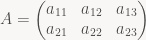, there’s two “canonical” ways to store it in memory (discounting fancier storage schemes such as tiled or Morton-order storage):

• Row-major storage traverses the matrix by rows, then within each row enumerates the columns. So our A would be stored in memory as a11, a12, a13, a21, a22, a23. This matches reading order in English and most other Western languages. Row-major storage order for 2D arrays is used by C / C++, the Borland dialects of Pascal, and pretty much any language that was designed since the mid-1970s and supports multidimensional arrays directly. (Several newer languages such as Java don’t support 2D arrays directly at all, opting instead to represent them as an 1D array of references to 1D arrays). It’s also the dominant storage order for images. The position of the element at row i, column j in the underlying 1D array is computed as i*stride + j, where stride is the number of elements stored per row, usually the width of the 2D array, but it can also be larger.
• Column-major storage traverses the matrix by columns, then enumerates the rows within each column. A would be stored in memory as a11, a21, a12, a22, a13, a23. Column-major storage is used by FORTRAN and hence by BLAS and LAPACK, the bread and butter of high-performance numerical computation. It is also used by GL for matrices (due to something of a historical accident), even though GL is a C-based library and all other types of 2D or higher-dimensional data in GL (2D/3D textures etc.) use row-major.

Let me reiterate: Both row and column major are about the way you layout 2D (3D, …) arrays in memory, which uses 1D addresses. In the example (and also in the following), I always write the row index first, followed by the column index, i.e. is the element of A in row i and column j, no matter which way it ends up being stored. By the same convention, I write “3×4 matrix” to denote a matrix with 3 rows and 4 columns, independent of memory layout.

Matrix multiplication

The next ingredient we need is matrix multiplication. If A and B are a and a matrix, respectively, their product C=AB is a matrix – note the middle dimension has to match between the two. The element in row i and column j of matrix C is computed as the dot product of the i-th row of A and the j-th column of B, or in formulas 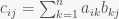. All this is standard stuff.

The important point to note here is that for a matrix product AB you always compute the dot product between rows of A and columns of B; there’s no disagreement here. This is how everyone does it, row-major layout or not.

Row and column vectors

So here’s where the confusion starts: a n-element vector can be interpreted as a matrix (a “typecast” if you will). Again, there’s two canonical ways to do this: either we stack the n numbers vertically into a matrix, which gives a column vector, or we arrange them horizontally, producing a matrix or row vector. Note that this has nothing to do with the storage layout; in both row and column major orders, row and column vectors are simply stored as a n-element 1D array.

Here’s where the confusion starts: To transform a vector by a matrix, you first need to convert the vector to a matrix (i.e. choose whether it’s supposed to be a column or row vector this time), then multiply the two. In the usual graphics setting, we have a 4×4 matrix T and a 4-vector v. Since the middle dimension in a matrix product must match, we can’t do this arbitrarily. If we write v as a 4×1 matrix (column vector), we can compute Tv but not vT. If v is instead a 1×4 matrix (row vector), only vT works and Tv leads to a “dimension mismatch”. For both column and row vectors, the result of that is again a column or row vector, respectively, which has repercussions: if we want to transform the result again by another matrix, again there’s only one place where we can legally put it. For column vectors, transforming a vector by T then S leads to the expression , so the matrix that represents “first T then S” is given by the matrix ST. For row vectors, we get , so the matrix for the concatenation of the two is given by TS. Small difference, big repercussions: whether you choose row or column vectors influences how you concatenate transforms.

GL fixed function is column-major and uses column vectors, whereas D3D fixed function was row-major and used row vectors. This has led a lot of people to believe that your storage order must always match the way you interpret vectors. It doesn’t. Another myth is that matrix multiplication order depends on whether you’re using row-major or column-major. It doesn’t: matrices are always multiplied the same way, and what that product matrix means depends on what type of vector you use, not what kind of storage scheme.

One more point: say you have two n-element vectors, u and v. There’s two ways to multiply these two together as a matrix product (yes, you can multiply two vectors): if u is a row vector and v is a column vector, the product is a 1×1 matrix, or just a single scalar, the dot product of the two vectors. This operation is the (matrix) inner product. If instead u is a column vector and v is a row vector, the result is a matrix, or outer product (actually the outer product can also be computed when the dimensions of u and v don’t match, but I ignore that case here). The outer product isn’t as common as its more famous cousin, but it does crop up in several places in Linear Algebra and is worth knowing about. I bring these two examples up to illustrate that you can’t just hand-wave away the issue of vector orientation entirely; you need both, and which one is which matters when the two interact.

With that cleared up, two comments: First, I recommend that you stick with whatever storage order is the default in your language/environment (principle of least surprise and all that), but it really doesn’t matter whether you pick row or column vectors – not in any deep sense, anyway. The difference between the two is purely one of notation (and convention). Second, there happens to be a very much dominant convention in maths, physics and really all the rest of the world except for Computer Graphics, and that convention is to use column vectors by default. For whatever reason, some of the very earliest CG texts chose to break with tradition and used row vectors, and ever since CG has been cursed with a completely unnecessary confusion about things such as matrix multiplication order. If you get to choose, I suggest you prefer column vectors. But whatever you do, make sure to document whatever you use in your code and stick with it, at least within individual components. In terms of understanding and debuggability, a single source file that uses two different vector math libraries with opposite conventions (or three – I’ve seen it happen) is a catastrophe. It’s a bug honeypot. Just say no, and fix it when you see it.

Buffer-centric IO

This is a small but nifty solution I discovered while working on IO code for Iggy. I don’t claim to have invented it – as usual in CS, this was probably first published in the 60s or 70s – but I definitely never ran across it in this form before, so it seems worth writing up. Small disclaimer up front: First, this describes a combination of techniques that are somewhat orthogonal, but they nicely complement each other, so I describe them at the same time. Second, it’s definitely not the best approach in every scenario, but it’s nifty and definitely worth knowing about. I’ve found it particularly useful when dealing with compressed data.

Setting

A lot of code needs to be able to accept data from different sources. Sometimes you want to load data from a file; sometimes it’s already in memory, or it’s a memory-mapped file (boils down to the same thing). If it comes from a file, you may have one file per item you want to load, or pack a bunch of related data into a “bundle” file. Finally, data may be compressed or encrypted.

If possible, the simplest solution is to just write your code to assume one such method and stick with it – the easiest usually being the “already in memory” option. This is fine, but can get problematic depending on the file format: for example, the SWF (Flash) files that Iggy loads are usually Deflate-compressed as a whole, and may contain chunks of image data that are themselves JPEG- or Deflate-compressed. Finally, Iggy wants all the data in its own format, not in the Flash file format, since even uncompressed Flash files involve a lot of bit-packing and implicit information that makes them awkward to deal with directly.

Ultimately, all we want to have in memory is our own data structures; but an implementation that expects all data to be decompressed to memory first will need a lot of extra memory (temporarily at least), which is problematic on memory-constrained platforms.

The standard solution is to get rid of the memory-centric view completely and instead implement a stream abstraction. For read-only IO (which is what I’ll be talking about here), a simple but typical (C++) implementation looks like this:

class SimpleStream {
public:
    virtual ErrorCode Read(U8 *buffer, U32 numBytes,
                           U32 *bytesActuallyRead) = 0;
};

Code that needs to read data takes a Stream argument and calls Read when necessary to fill its input buffers. You’ll find designs like this in most C++ libraries that handle at least some degree of IO.

Simple, right?

The problems

Actually, there’s multiple problems with this approach.

For example, consider the case where the file is already loaded into memory (or memory-mapped). The app expects data to land in buffer, so our Read implementation will end up having to do a memcpy or something similar. That’s unlikely to be a performance problem if it happens only once, but it’s certainly not pretty, and if you have multiple streams nested inside each other, the overhead keeps adding up.

Somewhat more subtly, there’s the business with numBytes and bytesActuallyRead. We request some number of bytes, but may get a different number of bytes back (anything between 0 and numBytes inclusive). So client code has to be able to deal with this. In theory, “stream producer” code can use this to make things simpler; to give an example, lots of compressed formats are internally subdivided into chunks (with sizes typically somewhere between 32KB and 1MB), and it’s convenient to write the code such that a single Read will never cross a chunk boundary. In practice, a lot of the “stream consumer” code ends up being written using memory or uncompressed file streams as input, and will implicitly assume that the only cases where “partial” blocks are returned are “end of file” or error conditions (because that’s all they ever see while developing the code). This behavior may be technically wrong, but it’s common, and the actual cost (slightly more complexity in the producer code) is low enough to not usually be worth making a stand about.

So we have an API where we frequently end up having to check for and deal with what’s basically the same boundary condition on both sides of the fence. That’s a bad sign.

Finally, there’s the issue of error handling. If we’re loading from memory, there’s basically only one error condition that can happen: unexpected end, when we’ve exhausted the input buffer even though we want to read more. But for a general stream, there’s all kinds of errors that can happen: end of file, yes, but also read errors from disk, timeouts when reading from a network file system, integrity-check errors, errors decompressing or decrypting a stream, and so on. Ideally, every single caller should check error codes (and perform error handling if necessary) all the time. Again, in practice, this is rarely done everywhere, and what error-handling code is there is often poorly tested.

The problem is that checking for and reacting to error conditions everywhere is inconvenient. One solution is using exception handling; but this is, at least among game developers, a somewhat controversial C++ feature. In the case of Iggy, which is written in C, it’s not even an option (okay, there is setjmp / longjmp, which we even use in some cases – though not for IO – but let’s not go there). A different option is to write the code such that error checking isn’t required after every Read call; if possible, this is usually much nicer to use.

A different approach

Without further ado, here’s a different stream abstraction:

struct BufferedStream {
    const U8 *start;      // Start of buffer.
    const U8 *end;        // (One past) end of buffer
                          // i.e. buffer_size = end-start.
    const U8 *cursor;     // Cursor in buffer. 
                          // Invariant: start <= cursor <= end.
    ErrorCode error;      // Initialized to NoError.

    ErrorCode (*Refill)(BufferedStream *s);
    // Pre-condition: cursor == end (buffer fully consumed).
    // Post-condition: start == cursor < end.
    // Always returns "error".
};

There’s 3 big conceptual differences here:

1. The buffer is owned and managed by the producer – the consumer does not get to specify where data ends up.
2. The Read function has been replaced with a Refill function, which reads in an unspecified amount of bytes – the one guarantee here is that at least one more byte will be returned, even in case of error; more about that later. Also note it’s a function pointer, not a virtual function. Again, there’s a good reason for that.
3. Instead of reporting an error code on every Read, there’s a persistent error variable – think errno (but local to the given stream, which avoids the serious problems that hamper the ‘real’ errno).

Note that this abstraction is both more general and more specific than the stream abstraction above: more general in the sense that it’s easy to implement SimpleStream::Read on top of the BufferedStream abstraction (I’ll get to that in a second), and more specific in the sense that all BufferedStream implementations are, by necessity, buffered (it might just be a one-byte-buffer, but it’s there). It’s also lower-level; the buffer isn’t encapsulated, it’s visible to client code. That turns out to be fairly important. Instead of elaborating, I’m gonna present a series of examples that demonstrate some of the strengths of this approach.

Example 1: all zeros

Probably the simplest implementation of this interface just generates an infinite stream of zeros:

static ErrorCode refillZeros(BufferedStream *s)
{
    static const U8 zeros[256] = { 0 };
    s->start = zeros;
    s->cursor = zeros;
    s->end = zeros + sizeof(zeros);
    return s->error;
}

static void initZeroStream(BufferedStream *s)
{
    s->Refill = refillZeros;
    s->error = NoError;
    s->Refill(s);
}

Not much to say here: whenever Refill is called, we reset the pointers to go over the same array of zeros again (the count of 256 is completely arbitrary; you could just as well use 1, but then you’d end up calling Refill a lot).

Example 2: stream from memory

For the next step up, here’s a stream that reads either directly from memory, or from a memory-mapped file:

static ErrorCode fail(BufferedStream *s, ErrorCode reason)
{
    // For errors: Set the error status, then continue returning
    // zeros indefinitely.
    s->error = reason;
    s->Refill = refillZeros;
    return s->Refill(s);
}

static ErrorCode refillMemStream(BufferedStream *s)
{
    // If this gets called, clients wants to read past the end of
    // the memory buffer, which is an error.
    return fail(s, ReadPastEOF);
}

static void initMemStream(BufferedStream *s, U8 *mem, size_t size)
{
    s->start = mem;
    s->cursor = mem;
    s->end = mem + size;
    s->error = NoError;
    s->Refill = refillMemStream;
}

The init function isn’t very interesting, but the Refill part deserves some explanation: As mentioned before, the client calls Refill when it’s finished with the current buffer and still needs more data. In this case, the “buffer” was all the data we had; therefore, if we ever try to refill, that means the client is trying to read past the end-of-file, which is an error, so we call fail, which first sets the error code. We then change the refill function pointer to refillZeros, our previous example: in other words, if the client tries to read past the end of file, they’ll get an infinite stream of zeros (satisfying our above invariant that Refill always returns at least one more byte). But the error flag will be set, and since refillZeros doesn’t touch it, it will stay the way it was.

In effect, making Refill a function pointer allows us to implicitly turn any stream into a state machine. This is a powerful facility, and it’s great for this kind of error handling and to deal with certain compressed formats (more later), but like any kind of state machine, it quickly gets more confusing than it’s worth if there’s more than a handful of states.

Anyway, there’s one more thing worth pointing out: there’s no copying here. A from-memory implementation of SimpleStream would need to do a memcpy (or something equivalent) in its Read function, but since we don’t let the client decide where the data ends up, we can just point it directly to the original bytes without doing any extra work. Because forwarding is effectively free, it makes it easy to decouple “framing” from data processing even in performance-critical code.

Example 3: parsing JPEG data

Case in point: JPEG data. JPEG files interleave compressed bitstream data and metadata. Metadata exists in several types and is denoted by a special code, a so-called “marker”. A marker consists of an all-1-bits byte (0xff) followed by a nonzero byte. Because the compressed bitstream can contain 0xff bytes too, they need to be escaped using the special code 0xff 0x00 (which is not interpreted as a marker). Thus code that reads JPEG data needs to look at every byte read, check if it’s 0xff, and if so look at the next byte to figure out whether it’s part of a marker or just an escape code. Having to do this in the decoder inner loop is both annoying (because it complicates the code) and slow (because it forces byte-wise processing and adds a bunch of branches). It’s much nicer to do it in a separate pass, and with this approach we can naturally phrase it as a layered stream (I’ll skip the initialization this time):

struct JPEGDataStream : public BufferedStream {
    BufferedStream *src; // Read from here
};

static ErrorCode refillJPEG_lastWasFF(BufferedStream *s);

static ErrorCode refillJPEG(BufferedStream *str)
{
    JPEGDataStream *j = (JPEGDataStream *)str;
    BufferedStream *s = j->src;

    // Refill if necessary and check for errors
    if (s->cursor == s->end) {
        if (s->Refill(s) != NoError)
            return fail(str, s->error);
    }

    // Find next 0xff byte (if any)
    U8 *next_ff = memchr(s->cursor, 0xff, s->end - s->cursor);
    if (next_ff) {
        // return bytes until 0xff,
        // continue with refillJPEG_lastWasFF.
        j->start = s->cursor;
        j->cursor = s->cursor; // EDIT typo fixed (was "current")
        j->end = next_ff;
        j->Refill = refillJPEG_lastWasFF;
        s->cursor = next_ff + 1; // mark 0xff byte as read
    } else {
        // return all of current buffer
        j->start = s->cursor;
        j->cursor = s->cursor;
        j->end = s->end;
        s->cursor = s->end; // read everything
    }
}

static ErrorCode refillJPEG_lastWasFF(BufferedStream *str)
{
    static const U8 one_ff[1] = { 0xff };
    JPEGDataStream *j = (JPEGDataStream *)str;
    BufferedStream *s = j->src;

    // Refill if necessary and check for errors
    if (s->cursor == s->end) {
        if (s->Refill(s) != NoError)
            return fail(str, s->error);
    }

    // Process marker type byte
    switch (*s->cursor++) {
    case 0x00:
        // Not a marker, just an escaped 0xff!
        // Return one 0xff byte, then resume regular parsing.
        j->start = one_ff;
        j->cursor = one_ff;
        j->end = one_ff + 1;
        j->Refill = refillJPEG;                        
        break;

        // Was a marker. Handle other cases here...

    case 0xff: // 0xff 0xff is invalid in JPEG
        return fail(str, CorruptedData);

    default:
        return fail(str, UnknownMarker);
    }
}

It’s a bit more code than the preceding examples, but it demonstrates how streams can be “layered” and also nicely shows how the implicit state machine can be useful.

Discussion

This clearly solves the first issue I raised – there’s no unnecessary copying going on. The interface is also really simple: Everything is in memory. Client code still has to deal with partial results, but because the client never gets to specify how much data to read in the first place, the interface makes it a lot clearer that handling this case is necessary. It also makes it a lot more common, which goes a long way towards making sure that it gets handled. Finally, error handling – this is only partially resolved, but the invariants have been picked to make the life of client code as easy as possible: All errors are “sticky”, so there’s no risk of “missing” an error if you do something else in between doing the read and checking for errors (a typical issue with errno, GetLastError and the like). And our error-“refill” functions still return data (albeit just zeros in these examples). These two things together mean that, in practice, you only really need to check for errors inside loops that might not terminate otherwise. In all other cases, you will fall through to the end of functions eventually; as long as you check the error code before you dispose of the stream, it will be noticed.

One really cool thing you can do with this type of approach (that I don’t want to discuss in full or with code because it would get lengthy and is really only interesting to a handful of people) is give the client pointers into the window in a LZ77-type compressor. This completely removes the need for any separate output buffers, saving a lot of copying and some small amount of memory. This is especially nice on memory-constrained targets like SPUs. In general, giving the producer (instead of the consumer) control over where the buffer is in memory allows producer code to use ring buffers (like a LZ77 window) completely transparently, which I think is pretty cool.

There’s a lot more that could be said about this, and initially I wanted to, but I didn’t want to make this too long; better have two medium-sized posts than one huge post that nobody reads to the finish. Besides, it means I can base a potential second post on actual questions I get, rather than having to guess what questions you might have, which I’m not very good at.

Checking for interval overlap

This’ll be a short post, based on a short exchange I recently had with a colleague at work (hey Per!). It’s about a few tricks for checking interval overlaps that aren’t as well-known as they should be. (Note: This post was originally written for AltDevBlogADay and posted there first).

The problem is very simple: We have two (closed) intervals and and want to find out if they overlap (i.e. have a non-empty intersection). So how would you do it? A simple solution can be obtained directly from the definition: we first compute the intersection of the two intervals, then check whether it’s non-empty.

The code for this is straightforward, and I’ve seen it many times in various codebases:

i0 = max(a0, b0); // lower bound of intersection interval
i1 = min(a1, b1); // upper bound of intersection interval
return i0 <= i1;  // interval non-empty?

However, doing the check this way without a native “max” operation (which most architectures don’t provide for at least some types) requires three comparisons, and sometimes some branching (if the architecture also lacks conditional moves). It’s not a tragedy, but neither is it particularly pretty.

Center and Extent

If you’re dealing with floating-point numbers, one reasonably well-known technique is using center and extents (actually half-extents) for overlap checks; this is the standard technique to check for collisions using Separating Axis Tests, for example. For closed and open intervals, the intuition here is that they can be viewed as 1D balls; instead of describing them by two points on their diameter, you can equivalently express them using their center and radius. It boils down to this:

float center0 = 0.5f * (a0 + a1);
float center1 = 0.5f * (b0 + b1);
float radius0 = 0.5f * (a1 - a0);
float radius1 = 0.5f * (b1 - b0);
return fabsf(center1 - center0) <= (radius0 + radius1);

This looks like a giant step back. Lots of extra computation! However, if you’re storing (open or closed) intervals, you might as well use the Center-Extent form in the first place, in which case all but the last line go away: a bit of math and just one floating-point compare, which is attractive when FP compares are expensive (as they often are). However, this mechanism doesn’t look like it’s easy to extend to non-floats; what about the multiply by 0.5? The trick here is to realize that all of the expressions involved are linear, so we might as well get rid of the scale by 0.5 altogether:

center0_x2 = a0 + a1;
center1_x2 = b0 + b1;
radius0_x2 = a1 - a0;
radius1_x2 = b1 - b0;
return abs(center1_x2 - center0_x2) <= (radius0_x2 + radius1_x2);

No scaling anymore, so this method can be applied to integer types as well as floating-point ones, provided there’s no overflow. In case you’re wondering, there’s efficient branch-less ways to implement abs() for both floats and integers, so there’s no hidden branches here. Of course you can also use a branch-less min/max on the original code snippet, but the end result here will be a bit nicer than that. Because eliminating common terms yields:

t0 = b1 - a0;
t1 = a1 - b0;
return abs(t0 - t1) <= (t0 + t1);

I thought this was quite pretty when I stumbled upon it for the first time. It only does one comparison, so it’s optimal in that sense, but it still involves a bit of arithmetic.

Rephrasing the question

The key to a better approach is inverting the sense of the question: instead of asking whether two intervals overlap, try to find out when they don’t. Now, intervals don’t have holes. So if two intervals and don’t overlap, that means that must be either fully to the left or fully to the right of on the real number line. Now, if is fully to the left of , that means in particular that b’s rightmost point must be to the left of a – that is, smaller than . And again, vice versa for the right side. So the two intervals don’t overlap if either or . Applying that to our original problem (which involves negating the whole expression using de Morgan's laws), this gives the following version of the interval overlap check:

return a0 <= b1 && b0 <= a1;

Which is about as simple as it gets.

Again, it’s not earth-shattering, but it’s not at all obvious from the original snippet above that the test can be done this way, so the longer version tends to come up quite often – even when the max and min operations use branches. It’s generally worthwhile to know all three forms so you can use them when appropriate – hence this post.

A trip through the Graphics Pipeline 2011, part 13

This post is part of the series “A trip through the Graphics Pipeline 2011”.

Welcome back to what’s going to be the last “official” part of this series – I’ll do more GPU-related posts in the future, but this series is long enough already. We’ve been touring all the regular parts of the graphics pipeline, down to different levels of detail. Which leaves one major new feature introduced in DX11 out: Compute Shaders. So that’s gonna be my topic this time around.

Execution environment

For this series, the emphasis has been on overall dataflow at the architectural level, not shader execution (which is explained well elsewhere). For the stages so far, that meant focusing on the input piped into and output produced by each stage; the way the internals work was usually dictated by the shape of the data. Compute shaders are different – they’re running by themselves, not as part of the graphics pipeline, so the surface area of their interface is much smaller.

In fact, on the input side, there’s not really any buffers for input data at all. The only input Compute Shaders get, aside from API state such as the bound Constant Buffers and resources, is their thread index. There’s a tremendous potential for confusion here, so here’s the most important thing to keep in mind: a “thread” is the atomic unit of dispatch in the CS environment, and it’s a substantially different beast from the threads provided by the OS that you probably associate with the term. CS threads have their own identity and registers, but they don’t have their own Program Counter (Instruction Pointer) or stack, nor are they scheduled individually.

In fact, “threads” in CS take the place that individual vertices had during Vertex Shading, or individual pixels during Pixel Shading. And they get treated the same way: assemble a bunch of them (usually, somewhere between 16 and 64) into a “Warp” or “Wavefront” and let them run the same code in lockstep. CS threads don’t get scheduled – Warps and Wavefronts do (I’ll stick with “Warp” for the rest of this article; mentally substitute “Wavefront” for AMD). To hide latency, we don’t switch to a different “thread” (in CS parlance), but to a different Warp, i.e. a different bundle of threads. Single threads inside a Warp can’t take branches individually; if at least one thread in such a bundle wants to execute a certain piece of code, it gets processed by all the threads in the bundle – even if most threads then end up throwing the results away. In short, CS “threads” are more like SIMD lanes than like the threads you see elsewhere in programming; keep that in mind.

That explains the “thread” and “warp” levels. Above that is the “thread group” level, which deals with – who would’ve thought? – groups of threads. The size of a thread group is specified during shader compilation. In DX11, a thread group can contain anywhere between 1 and 1024 threads, and the thread group size is specified not as a single number but as a 3-tuple giving thread x, y, and z coordinates. This numbering scheme is mostly for the convenience of shader code that addresses 2D or 3D resources, though it also allows for traversal optimizations. At the macro level, CS execution is dispatched in multiples of thread groups; thread group IDs in D3D11 again use 3D group IDs, same as thread IDs, and for pretty much the same reasons.

Thread IDs – which can be passed in in various forms, depending on what the shader prefers – are the only input to Compute Shaders that’s not the same for all threads; quite different from the other shader types we’ve seen before. This is just the tip of the iceberg, though.

Thread Groups

The above description makes it sound like thread groups are a fairly arbitrary middle level in this hierarchy. However, there’s one important bit missing that makes thread groups very special indeed: Thread Group Shared Memory (TGSM). On DX11 level hardware, compute shaders have access to 32k of TGSM, which is basically a scratchpad for communication between threads in the same group. This is the primary (and fastest) way by which different CS threads can communicate.

So how is this implemented in hardware? It’s quite simple: all threads (well, Warps really) within a thread group get executed by the same shader unit. The shader unit then simply has at least 32k (usually a bit more) of local memory. And because all grouped threads share the same shader unit (and hence the same set of ALUs etc.), there’s no need to include complicated arbitration or synchronization mechanisms for shared memory access: only one Warp can access memory in any given cycle, because only one Warp gets to issue instructions in any cycle! Now, of course this process will usually be pipelined, but that doesn’t change the basic invariant: per shader unit, we have exactly one piece of TGSM; accessing TGSM might require multiple pipeline stages, but actual reads from (or writes to) TGSM will only happen inside one pipeline stage, and the memory accesses during that cycle all come from within the same Warp.

However, this is not yet enough for actual shared-memory communication. The problem is simple: The above invariant guarantees that there’s only one set of accesses to TGSM per cycle even when we don’t add any interlocks to prevent concurrent access. This is nice since it makes the hardware simpler and faster. It does not guarantee that memory accesses happen in any particular order from the perspective of the shader program, however, since Warps can be scheduled more or less randomly; it all depends on who is runnable (not waiting for memory access / texture read completion) at certain points in time. Somewhat more subtle, precisely because the whole process is pipelined, it might take some cycles for writes to TGSM to become “visible” to reads; this happens when the actual read and write operations to TGSM occur in different pipeline stages (or different phases of the same stage). So we still need some kind of synchronization mechanism. Enter barriers. There’s different types of barriers, but they’re composed of just three fundamental components:

1. Group Synchronization. A Group Synchronization Barrier forces all threads inside the current group to reach the barrier before any of them may consume past it. Once a Warp reaches such a barrier, it will be flagged as non-runnable, same as if it was waiting for a memory or texture access to complete. Once the last Warp reaches the barrier, the remaining Warps will be reactivated. This all happens at the Warp scheduling level; it adds additional scheduling constraints, which may cause stalls, but there’s no need for atomic memory transactions or anything like that; other than lost utilization at the micro level, this is a reasonably cheap operation.
2. Group Memory Barriers. Since all threads within a group run on the same shader unit, this basically amounts to a pipeline flush, to ensure that all pending shared memory operations are completed. There’s no need to synchronize with resources external to the current shader unit, which means it’s again reasonably cheap.
3. Device Memory Barriers. This blocks all threads within a group until all memory accesses have completed – either direct or indirect (e.g. via texture samples). As explained earlier in this series, memory accesses and texture samples on GPUs have long latencies – think more than 600, and often above 1000 cycles – so this kind of barrier will really hurt.

DX11 offers different types of barriers that combine several of the above components into one atomic unit; the semantics should be obvious.

Unordered Access Views

We’ve now dealt with CS input and learned a bit about CS execution. But where do we put our output data? The answer has the unwieldy name “unordered access views”, or UAVs for short. An UAV seems somewhat similar to render targets in Pixel Shaders (and UAVs can in fact be used in addition to render targets in Pixel Shaders), but there’s some very important semantic differences:

• Most importantly, as the same suggests, access to UAVs is “unordered”, in the sense that the API does not guarantee accesses to become visible in any particular order. When rendering primitives, quads are guaranteed to be Z-tested, blended and written back in API order (as discussed in detail in part 9 of this series), or at least produce the same results as if they were – which takes substantial effort. UAVs make no such effort – UAV accesses happen immediately as they’re encountered in the shader, which may be very different from API order. They’re not completely unordered, though; while there’s no guaranteed order of operations within an API call, the API and driver will still collaborate to make sure that perceived sequential ordering is preserved across API calls. Thus, if you have a complex Compute Shader (or Pixel Shader) writing to an UAV immediately followed by a second (simpler) CS that reads from the same underlying resource, the second CS will see the finished results, never some partially-written output.
• UAVs support random access. A Pixel Shader can only write to one location per render target – its corresponding pixel. The same Pixel Shader can write to arbitrary locations in whatever UAVs it has bound.
• UAVs support atomic operations. In the classic Pixel Pipeline, there’s no need; we guarantee there’s never any collisions anyway. But with the free-form execution provided by UAVs, different threads might be trying to access a piece of memory at the same time, and we need synchronization mechanisms to deal with this.

So from a “CPU programmer”‘s point of view, UAVs correspond to regular RAM in a shared-memory multiprocessing system; they’re windows into memory. More interesting is the issue of atomic operations; this is one area where current GPUs diverge considerably from CPU designs.

Atomics

In current CPUs, most of the magic for shared memory processing is handled by the memory hierarchy (i.e. caches). To write to a piece of memory, the active core must first assert exclusive ownership of the corresponding cache line. This is accomplished using what’s called a “cache coherency protocol”, usually MESI and descendants. The details are tangential to this article; what matters is that because writing to memory entails acquiring exclusive ownership, there’s never a risk of two cores simultaneously trying to write to the some location. In such a model, atomic operations can be implemented by holding exclusive ownership for the duration of the operation; if we had exclusive ownership for the whole time, there’s no chance that someone else was trying to write to the same location while we were performing the atomic operation. Again, the actual details of this get hairy pretty fast (especially as soon as things like paging, interrupts and exceptions get involved), but the 30000-feet-view will suffice for the purposes of this article.

In this type of model, atomic operations are performed using the regular Core ALUs and load/store units, and most of the “interesting” work happens in the caches. The advantage is that atomic operations are (more or less) regular memory accesses, albeit with some extra requirements. There’s a couple of problems, though: most importantly, the standard implementation of cache coherency, “snooping”, requires that all agents in the protocol talk to each other, which has serious scalability issues. There are ways around this restriction (mainly using so-called Directory-based Coherency protocols), but they add additional complexity and latency to memory accesses. Another issue is that all locks and memory transactions really happen at the cache line level; if two unrelated but frequently-updated variables share the same cache line, it can end up “ping-ponging” between multiple cores, causing tons of coherency transactions (and associated slowdown). This problem is called “false sharing”. Software can avoid it by making sure unrelated fields don’t fall into the same cache line; but on GPUs, neither the cache line size nor the memory layout during execution is known or controlled by the application, so this problem would be more serious.

Current GPUs avoid this problem by structuring their memory hierarchy differently. Instead of handling atomic operations inside the shader units (which again raises the “who owns which memory” issue), there’s dedicated atomic units that directly talk to a shared lowest-level cache hierarchy. There’s only one such cache, so the issue of coherency doesn’t come up; either the cache line is present in the cache (which means it’s current) or it isn’t (which means the copy in memory is current). Atomic operations consist of first bringing the respective memory location into the cache (if it isn’t there already), then performing the required read-modify-write operation directly on the cache contents using a dedicated integer ALU on the atomic units. While an atomic unit is busy on a memory location, all other accesses to that location will stall. Since there’s multiple atomic units, it’s necessary to make sure they never try to access the same memory location at the same time; one easy way to accomplish this is to make each atomic unit “own” a certain set of addresses (statically – not dynamically as with cache line ownership). This is done by computing the index of the responsible atomic unit as some hash function of the memory address to be accessed. (Note that I can’t confirm this is how current GPUs do; I’ve found little detail on how the atomic units work in official docs).

If a shader unit wants to perform an atomic operation to a given memory address, it first needs to determine which atomic unit is responsible, wait until it is ready to accept new commands, and then submit the operation (and potentially wait until it is finished if the result of the atomic operation is required). The atomic unit might only be processing one command at a time, or it might have a small FIFO of outstanding requests; and of course there’s all kinds of allocation and queuing details to get right so that atomic operation processing is reasonably fair so that shader units will always make progress. Again, I won’t go into further detail here.

One final remark is that, of course, outstanding atomic operations count as “device memory” accesses, same as memory/texture reads and UAV writes; shader units need to keep track of their outstanding atomic operations and make sure they’re finished when they hit device memory access barriers.

Structured buffers and append/consume buffers

Unless I missed something, these two buffer types are the last CS-related features I haven’t talked about yet. And, well, from a hardware perspective, there’s not that much to talk about, really. Structured buffers are more of a hint to the driver-internal shader compiler than anything else; they give the driver some hint as to how they’re going to be used – namely, they consist of elements with a fixed stride that are likely going to be accessed together – but they still compile down to regular memory accesses in the end. The structured buffer part may bias the driver’s decision of their position and layout in memory, but it does not add any fundamentally new functionality to the model.

Append/consume buffers are similar; they could be implemented using the existing atomic instructions. In fact, they kind of are, except the append/consume pointers aren’t at an explicit location in the resource, they’re side-band data outside the resource that are accessed using special atomic instructions. (And similarly to structured buffers, the fact that their usage is declared as append/consume buffer allows the driver to pick their location in memory appropriately).

Wrap-up.

And… that’s it. No more previews for the next part, this series is done :), though that doesn’t mean I’m done with it. I have some restructuring and partial rewriting to do – these blog posts are raw and unproofed, and I intend to go over them and turn it into a single document. In the meantime, I’ll be writing about other stuff here. I’ll try to incorporate the feedback I got so far – if there’s any other questions, corrections or comments, now’s the time to tell me! I don’t want to nail down the ETA for the final cleaned-up version of this series, but I’ll try to get it down well before the end of the year. We’ll see. Until then, thanks for reading!

Migrating Thunderbird profiles: A story in three acts

Prologue

This is a slight bit of a departure from the usual themes in this blog, but I thought it was interesting enough to write it up anyway. It also makes for a nice break from the Trip through the Graphics Pipeline series that’s been dominating this blog recently (conclusion coming Real Soon Now – and there’s 4 other queued up articles in various stages of completion, we’ll see what comes of that).

Act I

in which the protagonist fails at performing a seemingly simple task.

My laptop was getting a bit long in the tooth – the way that these things go. Battery charges don’t last as long as they used to – I’m used to that. WiFi grows a bit erratic – well, whatever, it never was that stable anyway. Windows getting a bit sluggish? Happens. Fans don’t work properly anymore so CPU stays permanently down-clocked and I can’t even watch videos without stutters anymore, HD starts making slightly worrying noises, Windows Update gets stuck trying to install one patch on every single shutdown and crashes? Okay, so maybe it was time to buy a new laptop after all. Which I promptly did a few weeks ago.

Now, the way new hardware usually goes for me is I buy it, maybe put it together, make sure that it works properly, then don’t do much with it for a while, and finally decide to spend a weekend to migrating data over from the predecessor machine. Now, that “don’t do much with it for a while” phase can last for a long time – when I first got a 64-bit machine, I set it up then didn’t touch it again for the next 3 months; in this case it wasn’t that extreme, but it still took me over a week until I started setting up the new machine; that was last weekend.

For the most part, this was exactly as boring as you would expect – installing a bunch of programs, copying over data, the works. However, it got a bit more interesting when I tried to transfer my Thunderbird profile (including mails) over from my previous machine. If you’ve never done this, it’s an “interesting” user experience, because to this date the Thunderbird authors seem to think that this problem is sufficiently rare and esoteric that it doesn’t need to be solved by their mail client directly (…no comment). The unofficial way to do this is to either locate and copy your profile directory manually, or to use MozBackup, a third-party tool that locates the profile directory for you and packs up all its contents into one file that can then be transferred to (and restored on) the target machine. I picked the latter option, because the Thunderbird profile is spread across multiple directories (…why?!?) and I vaguely remembered that the last time I had tried to do this manually, I ran into some weird issue where part of my profile wasn’t where I expected it to be. So I figured, let the specialized tool deal with it this time!

Given the title of this post and the fact that we’re still in Act I, it shouldn’t come as much of a surprise that this did not, in fact, work properly. Well, to be fair, it mostly worked – my main private mail account, all its associated filter rules, and two other “legacy” POP3 accounts that I check maybe once every 6 months came over just fine. However, my work email account did not work properly. It was added, the screen/user names as well as the server settings were all correct, but Thunderbird just wouldn’t display any of its folders no matter what I did. Well, since this was an IMAP account, I figured I might as well delete it and set it up anew – all the mails were on the server anyway. So that’s what I did – only to realize that I wasn’t sure about the password anymore; I had last entered it over a year ago. I did have it written down on a post-it in my office when I started at RAD, but I’ve switched offices two times since then, and that post-it was nowhere to be found. Anyway, I created a new mail account for my work address, entered the password the way I remembered and… nothing happened. Absolutely nothing. Again, no folders, no nothing. Not even signs of communication with the server.

I figured that something must be going wrong with the password authentication, but since Thunderbird didn’t pop up any error messages, I wasn’t sure where to start looking. And after a day spent setting up a machine, I didn’t feel like debugging either. So I decided to leave it alone for awhile.

Act II

in which passwords are changed and bugs in the mail admin interface are discovered.

On Wednesday I decided that I should really get this resolved before the weekend, so I asked around whether we had the passwords written down somewhere (and got the Only Right Answer: no, we didn’t!) and if not, whether my password could be reset to a new value – it could, but only my boss had the necessary password for our mail system, so it took another day for the password change to happen, which was today.

It was a simple plan: Jeff (my boss) would just change my mail password and give me the new one.

Well, it was a partial success. Jeff indeed changed my password and gave me a new one – except it didn’t work. Some triple-checking and experimenting later, I decided that he had probably made a typo in either the new password or the string he sent me. So I went to his office and told him so – “no, I definitely gave you the right password!”. He went to the mail admin interface, tried to log in with me username and the new password, and… it didn’t work. First response: “okay, did I manage to mistype that the same way twice when I changed the password?”. So he changed the password again to the intended value – nope, didn’t work this time either.

New theory: Since the new password was more like a passphrase and involved SeveralWordsInCamelCase, it was quite long; my old password had been 10 characters, whereas the new password might exceed whatever internal limit the system had. I’d had that suspicion before and tried several prefixes of the password with various lengths on my login attempts, but none of them worked either. But this time, Jeff changed the password to something shorter, and indeed, logging in worked fine now. Great – evidently there was a limit on password length, but the admin interface didn’t warn about it or produce any error – it just changed the password anyway (it’s unclear what it changed it to) and happily chugged along. Great.

Anyway, I could read my work mails at work again, which was good enough for the moment. As I discovered a bit later though, it did not fix the Thunderbird mail issues I was having; even with a password that I knew worked on my office PC (using the exact same server settings and version of Thunderbird), IMAP wouldn’t work at all on my new laptop. And as the curtain falls for Act II, I leave you with one simple question to ponder: What if Jeff had tried to use the long password for the admin account instead of mine?

Act III

in which experiments are conducted and the terrible truth is revealed.

When the password that I knew was right still failed in my Thunderbird setup, I knew that something deeper was wrong. So it was time to switch into experimentation mode: rename my profile directory so Thunderbird couldn’t find it, uninstall Thunderbird, re-install it, and set up the RAD email account on a fresh, pristine installation of Thunderbird.

And voilá, it worked just fine.

Okay, now I had a fresh IMAP account that worked. So I figured, hey, let MozBackup restore settings for my other accounts from the backed up profile again and I’m set, right? Wrong. MozBackup can’t do that. It’s all or nothing – you can backup/restore a whole profile, but not individual accounts in it, and restoring overwrites everything in the profile include whatever new accounts you may have set up. Great.

Plan B: I still had the original backup file that I used to transfer the mails over to the new machine. MozBackup will not let you restore individual accounts, but it will let you select what kind of information to restore. I figured that something was wrong with the settings, so instead of restoring everything, I kept it to the bare bones (just Emails and the Address Book). Nope, even just restoring these two things alone, I could neither use the restored RAD IMAP account nor set up a new IMAP account.

I decided to check the error console. There was a bunch of error spew in there all right, but it was completely useless, consisting of a few hex values and a trace to some JavaScript function that also didn’t prove helpful in determining what was going on. Googling for the error message turned up nothing interesting – there was a reference to a bug in some old Thunderbird version, but it had (according to the ticket anyway) been fixed long ago, and indeed I can confirm that the patch in question had been applied, since that was the code I was getting the error message from. All I got from that line of investigation was that it was trying (and failing) to enumerate mail folders for that account – yes, indeed, I could see that by myself.

Okay, Plan C: Go back to the original profile and try to figure out what’s wrong by myself. I didn’t really know where to start, so I just grepped for the mail server name in the main profile to directory to see where it would turn up.

First, I got a whole bunch of hits in a file called panacea.dat. So I looked at that file – WTF? It was full of path names from my old machine! (how to tell? The paths start with C:\Dokumente und Einstellungen, which is the German equivalent to the XP-era C:\Documents and Settings; the new Laptop is running English Windows 7, and that path doesn’t exist). In fact, it was full of path names to mail folders for old mail accounts, some of which I deleted 6 years ago. Some googling later, I learn that panacea.dat is just a cache for the location of mail folders. So I should be able to just delete it, right? Well, rename it, anyway – never ever randomly delete files in this kind of situation! And indeed, after restarting Thunderbird I was rewarded with a shiny, new, 17k panacea.dat (instead of the old 77k one) that only contained references to directories that actually existed on my machine. Progress! Sadly, it didn’t solve the problem, though; my RAD account still wouldn’t work.

Okay, what else showed up in the grep I did earlier? Next promising target was prefs.js. And, indeed: paydirt! First interesting thing I found in that file was this:

user_pref("mail.root.imap", "C:\\DOCUMENTS AND SETTINGS\\FG\\APPLICATION DATA\\Thunderbird\\Profiles\\Default User\\rtq40szi.slt\\ImapMail");
user_pref("mail.root.imap-rel", "[ProfD]../../../../../../DOCUMENTS AND SETTINGS/FG/APPLICATION DATA/Thunderbird/Profiles/Default User/rtq40szi.slt/ImapMail");
user_pref("mail.root.none", "C:\\DOCUMENTS AND SETTINGS\\FG\\APPLICATION DATA\\Thunderbird\\Profiles\\Default User\\rtq40szi.slt\\Mail");
user_pref("mail.root.none-rel", "[ProfD]../../../../../../DOCUMENTS AND SETTINGS/FG/APPLICATION DATA/Thunderbird/Profiles/Default User/rtq40szi.slt/Mail");
user_pref("mail.root.pop3", "C:\\DOCUMENTS AND SETTINGS\\FG\\APPLICATION DATA\\Thunderbird\\Profiles\\Default User\\rtq40szi.slt\\Mail");
user_pref("mail.root.pop3-rel", "[ProfD]Mail");

WTF? Absolute path names? And using the English version, of the path names, no less! Remember this profile came from a machine running a German Windows XP. More importantly, the relative version of the root for POP3 is set up correctly, whereas for “none” and IMAP, it’s effectively an absolute path, and it means it’ll try to use the “Documents and Settings” version even on the German Windows XP that was on the source machine. Also, rtq40szi.slt is not the unique ID for the profile on the source machine – it used 8z9cx5rb.default! What the hell was going on?

A bit later in the file, there were paths for the various identities. For reference, here are the corresponding paths for my main private mail address:

user_pref("mail.server.server1.directory", "C:\\Dokumente und Einstellungen\\fg\\Anwendungsdaten\\Thunderbird\\Profiles\\8z9cx5rb.default\\Mail\\mail.gmx.net");
user_pref("mail.server.server1.directory-rel", "[ProfD]Mail/mail.gmx.net");

Note that this time, the absolute directory actually exists on the source machine, it’s using the right profile ID, and the relative path makes sense. Compare to the path for my work mail address:

user_pref("mail.server.server6.directory", "C:\\DOCUMENTS AND SETTINGS\\FG\\APPLICATION DATA\\Thunderbird\\Profiles\\Default User\\rtq40szi.slt\\ImapMail\\mail.radgametools.com");
user_pref("mail.server.server6.directory-rel", "[ProfD]../../../../../../DOCUMENTS AND SETTINGS/FG/APPLICATION DATA/Thunderbird/Profiles/Default User/rtq40szi.slt/ImapMail/mail.radgametools.com");

And another WTF – this time it’s using the English version of the directory name again, the wrong profile ID, and the relative path is completely screwed up again!

At that point I decided to double-check on the source machine. And indeed, I did have c:\DOCUMENTS AND SETTINGS\FG\... (all caps for some reason) that contained exactly my work email identity and nothing else.

Once I figured that out, I just copied the contents of that profile directory into the main profile directory on my new laptop. I then fixed up all the paths in prefs.js (read: I deleted the absolute path references and replaced the relative ones with sane values). And tada – now my work email account worked. Problem finally solved!

Epilogue

Okay, so there’s one unanswered question: How did the profile stuff get fucked up like that in the first place? To be honest, I’m not sure; I’ve been using Thunderbird since mid-2004 (that was before 1.0) and migrated it between several machines over that time. However, I can guess: Even though I’m from Germany, I’ve been mostly using English Windows versions for a long time. All the SW I use on a daily basis comes in English, and using English SW on a German Windows results in things like Message Boxes with English text and German “Ja” / “Nein” (Yes / No) buttons. And we can’t have that, can we? Right. So given the choice, I’ve been buying English versions of Windows for a long time. But sometimes you don’t have a choice – when buying my old laptop, for instance, which came with a German OEM version of Windows and had no option to change the language.

So when I originally moved the Thunderbird profile to my Laptop, it was from an English version of Windows. At that point, my profile had several POP3 accounts still in use, so the stored relative root path for POP3 accounts ([ProfD]Mail) worked. I did not, however, have an active IMAP account at that point in time (I had deleted my University IMAP account some months earlier). Thus my profile contained no “ImapMail” folder – and since neither the absolute nor relative root path contained a valid directory name, Thunderbird apparently decided to trust the stored absolute path name and set the new relative path from it (which is how the whole ../../../../../../DOCUMENTS AND SETTINGS business got started).

This didn’t matter for the next one and a half years, during which I used no IMAP account. However, when I started at RAD last year, I added my work mail address as an IMAP account, at which point the C:\DOCUMENTS AND SETTINGS directory presumably got created on the German XP laptop. This being XP, you could still create directories at the root of the drive without admin privileges.

Now, the settings imported to the new laptop contained all the broken IMAP root directory settings from the profile – but this being Windows 7, you can’t just create a “Documents and Settings” in the root directory this time. So Thunderbird knew where it wanted to create its profile directory, but couldn’t, and therefore it couldn’t set up its mailbox files, and therefore I couldn’t see any mails. Awesome.

What really pisses me off about this whole episode is that a) Thunderbird doesn’t complain when profile data is stored outside the profile root directory (that should be a red flag right there!), b) Thunderbird stores absolute path names anywhere in the first place (why?!?), and c) despite there having to be at least half a dozen failed system calls on the way there, the only actual error that gets reported in any visible fashion is from some stupid JavaScript frontend thing. And not only is that error message hidden in a place where an average user would probably never find it, it’s also completely indecipherable even if you know where to look.

A trip through the Graphics Pipeline 2011, part 12

This post is part of the series “A trip through the Graphics Pipeline 2011”.

Welcome back! This time, we’ll look into what is perhaps the “poster boy” feature introduced with the D3D11 / Shader 5.x hardware generation: Tessellation. This one is interesting both because it’s a fun topic, and because it marks the first time in a long while that a significant user-visible component has been added to the graphics pipeline that’s not programmable.

Unlike Geometry Shaders, which are conceptually quite easy (it’s just a shader that sees whole primitives as opposed to individual vertices), the topic of “Tessellation” requires some more explanation. There’s tons of ways to tessellate geometry – to name just the most popular ones, there’s Spline Patches in dozens of flavors, various types of Subdivision Surfaces, and Displacement Mapping – so from the bullet point “Tessellation” alone it’s not at all obvious what services the GPU provides us with, and how they are implemented.

To describe how hardware tessellation works, it’s probably easiest to start in the middle – with the actual primitive tessellation step, and the various requirements that apply to it. I’ll get to the new shader types (Hull Shaders and Domain Shaders in D3D11 parlance, Tessellation Control Shader and Tessellation Evaluation Shader in OpenGL 4.0 lingo) later.

Tessellation – not quite like you’d expect

Tessellation as implemented by Shader 5.x class HW is of the “patch-based” variety. Patch types in the CG literature are mostly named by what kind of function is used to construct the tessellated points from the control points (B-spline patches, Bézier triangles, etc.). But we’ll ignore that part for now, since it’s handled in the new shader types. The actual fixed-function tessellation unit deals only with the topology of the output mesh (i.e. how many vertices there are and how they’re connected to each other); and it turns out that from this perspective, there’s basically only two different types of patches: quad-based patches, which are defined on a parameter domain with two orthogonal coordinate axes (which I’ll call u and v here, both are in [0,1]) and usually constructed as a tensor product of two one-parameter basis functions, and triangle-based patches, which use a redundant representation with three coordinates (u, v, w) based on barycentric coordinates (i.e. ). In D3D11 parlance, these are the “quad” and “tri” domains, respectively. There’s also an “isoline” domain which instead of a 2D surface produces one or multiple 1D curves; I’ll treat it the same way as I did lines and point primitives throughout this series: I acknowledge its existence but won’t go into further detail.

Tessellated primitives can be drawn naturally in their respective domain coordinate systems. For quads, the obvious choice of drawing the domain is as a unit square, so that’s what I’ll use; for triangles, I’ll use an equilateral triangle to visualize things. Here’s the coordinate systems I’ll be using in this post with both the vertices and edges labeled:

Anyway, both triangles and quads have what I would consider a “natural” way to tessellate them, depicted below. But it turns out that’s not actually the mesh topology you get.

Here’s the actual meshes that the tessellator will produce for the given input parameters:

For quads, this is (roughly) what we’re expecting – except for some flipped diagonals, which I’ll get to in a minute. But the triangle is a completely different beast. It’s got a very different topology from the “natural” tessellation I showed above, including a different number of vertices (12 instead of 10). Clearly, there’s something funny going on here – and that something happens to be related to the way transitions between different tessellation levels are handled.

Making ends meet

The elephant in the room is handling transitions between patches. Tessellating a single triangle (or quad) is easy, but we want to be able to determine tessellation factors per-patch, because we only want to spend triangles where we need them – and not waste tons of triangles on some distant (and possibly backface-culled) parts of the mesh. Additionally, we want to be able to do this quickly and ideally without extra memory usage; that means a global fix-up post-pass or something of that caliber is out of the question.

The solution – which you’ve already encountered if you’ve written a Hull or Domain shader – is to make all of the actual tessellation work purely local and push the burden of ensuring watertightness for the resulting mesh down to the shaders. This is a topic all by itself and requires, among other things, great care in the Domain Shader code; I’ll skip all the details about expression evaluation in shaders and stick with the basics. The basic mechanism is that each patch has multiple tessellation factors (TFs), which are computed in the Hull Shader: one or two for the actual inside of the patch, plus one for each edge. The TFs for the inside of the patch can be chosen freely; but if two patches share an edge, they’d better compute the exact same TFs along that edge, or there will be cracks. The hardware doesn’t care – it will process each patch by itself. If you do everything correctly, you’ll get a nice watertight mesh, otherwise – well, that’s your problem. All the HW needs to make sure is that it’s possible to get watertight meshes, preferably with reasonable efficiency. That by itself turns out to be tricky in some places; I’ll get to that later.

So, here are some new reference patches – this time with different TFs along each edge so we can see how that works:

I’ve colored the areas influenced by the different edge tessellation factors; the uncolored center part in the middle only depends on the inside TFs. In these images, the u=0 (yellow) edge has a TF of 2, the v=0 (green) edge has a TF of 3, the u=1 / w=0 (pink) edge has a TF of 4, and the v=1 (quad only, cyan) edge has a TF of 5 – exactly the number of vertices along the corresponding outer edge. As should be obvious from these two images, the basic building block for topology is just a nice way to stitch two subdivided edges with different number of vertices to each other. The details of this are somewhat tricky, but not particularly interesting, so I won’t go into it.

As for the inside TFs, quads are fairly easy: The quad above has an inside TF of 3 along u and 4 along v. The geometry is basically that of a regular grid of that size, except with the first and last rows/columns replaced by the respective stitching triangles (if any edge has a TF of 1, the resulting mesh will have the same structure as if the inside TFs for u/v were both 2, even if they’re smaller than that). Triangles are a bit more complicated. Odd TFs we’ve already seen – for a TF of , they produce a mesh consisting of concentric rings, the innermost of which is a single triangle. For even TFs, we get concentric rings with a center vertex instead of a center triangle. Below is an image of the simplest even case, , which consists just of edge stitches plus the center vertex.

Finally, when triangulating quads, the diagonal is generally chosen to point away from the center of the patch (in the domain coordinate space), with a consistent tie-breaking rule. This is simply to ensure maximum rotational symmetry of the resulting meshes – if there’s extra degrees of freedom, might as well use them!

Fractional tessellation factors and overall pipeline flow

So far, I’ve only talked about integer TFs. In two of the so-called “partitioning types”, namely “Integer” and “Pow2”, that’s all the Tessellator sees. If the shader generates a non-integer (or, respectively, non-power-of-2) TF, it will simply get rounded up to the next acceptable value. More interesting are the remaining two partitioning types: Fractional-odd and Fractional-even tessellation. Instead of jumping from tessellation factor to tessellation factor (which would cause visible pops), new vertices start out at the same position as an existing vertex in the mesh and then gradually move to their new positions as the TF increases.

For example, with fractional-odd tessellation, if you were to use an inner TF of 3.001 for the above triangle, the resulting mesh would look very much like the mesh for a TF of 3 – but topologically, it’d be the same as if the TF was 5, i.e. it’s a patch with 3 concentric rings, even though the middle ring is very narrow. Then as the TF gets closer to 5, the middle ring expands until it is eventually at its final position for TF 5. Once you raise the TF past 5, the mesh will be topologically the same as is the TF was 7, but again with a number of almost-degenerate triangles in the middle, and so forth. Fractional-even tessellation uses the same principle, just with even TFs.

The output of the tessellator then consists of two things: First, the positions of the tessellated vertices in domain coordinates, and second, the corresponding connectivity information – basically an index buffer.

Now, with the basic function of the fixed-function tessellator unit explained, let’s step back and see what we need to do to actually churn out primitives: First, we need to input a bunch of input control points comprising a patch into the Hull Shader. The HS then computes output control points and “patch constants” (both of which get passed down to the Domain Shader), plus all Tessellation Factors (which are essentially just more patch constants). Then we run the fixed-function tessellator, which gives us a bunch of Domain Positions to run the Domain Shader at, plus the associated indices. After we’ve run the DS, we then do another round of primitive assembly, and then send the primitives either down to the GS pipeline (if it’s active) or Viewport transform, Clip and Cull (if not).

So let’s look a bit into the HS stage.

Hull Shader execution

Like Geometry Shaders, Hull Shaders work on full (patch) primitives as input – with all the input buffering headaches that causes. How much of a headache entirely depends on the type of input patch. If the patch type is something like a cubic Bézier patch, we need 4×4 = 16 input points per patch and might just produce a single quad of output (or even none at all, if the patch is culled); clearly, that’s a somewhat awkward amount of data to work with, and doesn’t lend itself to very efficient shading. On the other hand, if tessellation takes plain triangles as input (which a lot of people do), input buffering is pretty tame and not likely to be a source of problems or bottlenecks.

More importantly, unlike Geometry Shaders (which run for every primitive), Hull Shaders don’t run all that often – they run once per patch, and as long as there’s any actual tessellation going on (even at modest TFs), we have way less patches than we have output triangles. In other words, even when HS input is somewhat inefficient, it’s less of an issue than in the GS case simply because we don’t hit it that often.

The other nice attribute of Hull Shaders is that, unlike Geometry Shaders, they don’t have a variable amount of output data; they produce a fixed amount of control points, each which a fixed amount of associated attributes, plus a fixed amount of patch constants. All of this is statically known at compile time; no dynamic run-time buffer management necessary. If we Hull Shade 16 hulls at a time, we know exactly where the data for each hull will end up before we even start executing the shader. That’s definitely an advantage over Geometry Shaders; for lots of Geometry Shaders, it’s possible to know statically how many output vertices will be generated (for example because all the control flow leading to emit / cut instructions can be statically evaluated at compile time), and for all of them, there’s a guaranteed maximum number of output vertices, but for HS, we have a guaranteed fixed amount of output data, no additional analysis required. In short, there’s no problems with output buffer management, other than the fact that, again depending on the primitive type, we might need lots of output buffer space which limits the amount of parallelism we can achieve (due to memory/register constraints).

Finally, Hull Shaders are somewhat special in the way they are compiled in D3D11; all other shader types basically consist of one block of code (with some subroutines maybe), but Hull Shaders are generated factored into multiple phases, each of which can consist of multiple (independent) threads of execution. The details are mainly of interest to driver and shader compiler programmers, but suffice it to say that your average HS comes packaged in a form that exposes lots of latent parallelism, if there is any. It certainly seems like Microsoft was really keen to avoid the bottlenecks that plague Geometry Shaders this time around.

Anyway, Hull Shaders produce a bunch of output per patch; most of it is just kept around until the corresponding Domain Shaders run, except for the TFs, which get sent to the tessellator unit. If any of the TFs are less than or equal to zero (or NaN), the patch is culled, and the corresponding control points and patch constants silently get thrown away. Otherwise, the Tessellator (which implements the functionality described above) kicks in, reads the just-shaded patches, and starts churning out domain point positions and triangle indices, and we need to get ready for DS execution.

Domain Shaders

Just like for Vertex Shading way back, we want to gather multiple domain vertices into one batch that we shade together and then pass on the PA. The fixed-function tessellator can take care of this: “just” handle it along with producing vertex positions and indices (I put the “just” in quotes here because this does involve some amount of bookkeeping).

In terms of input and output, Domain Shaders are very simple indeed: the only input they get that actually varies per vertex is the domain point u and v coordinates (w, when used, doesn’t need to be computed or passed in by the tesselator; since , it can be computed as ). Everything else is either patch constants, control points (all of which are the same across a patch) or constant buffers. And output is basically the same as for Vertex Shaders.

In short, once we get to the DS, life is good; the data flow is almost as simple as for VS, which is a path we know how to run efficiently. This is perhaps the biggest advantage of the D3D11 tessellation pipeline over Geometry Shaders: the actual triangle amplification doesn’t happen in a shader, where we waste precious ALU cycles and need to keep buffer space for a worst-case estimate of vertices, but in a localized element (the tessellator) that is basically a state machine, gets very little input (a few TFs) and produces very compact output (effectively an index buffer, plus a 2D coordinate per output vertex). Because of this, we need way less memory for buffering, and can keep our Shader Units busy with actual shading work instead of housekeeping.

And that’s it for this post – next up: Compute Shaders, aka the final part in my original outline for this series! Until then.

Final remarks

As usual, I cut a few corners. There’s the “isoline” patch type, which I didn’t go into at all (if there’s any demand for this, I can write it up). The Tessellator has all kinds of symmetry and precision requirements; as far as vertex domain positions are concerned, you can basically expect bit-exact results between the different HW vendors, because the D3D11 spec really nails this bit down. What’s intentionally not nailed down is the order in which vertices or triangles are produced – an implementation can do what it wants there, provided it does so consistently (i.e. the same input has to produce the same output, always). There’s a bunch of subtle constraints that go into this too – for example, all domain positions written by the Tessellator need to have both u and 1-u (and also v and 1-v) exactly representable as float; there’s a bunch of necessary conditions like this so that Domain Shaders can then produce watertight meshes (this rule in particular is important so that a shared edge AB between two patches, which is AB to one patch and BA to the other, can get tessellated the same way for both patches).

Writing Domain Shaders so they actually can’t produce cracks is tricky and requires great care; I intentionally sidestep the topic because it’s outside the scope of this series. Another much more trivial issue that I didn’t mention is the winding order of triangles generated by the Tessellator (answer: it’s up to the App – both clockwise and counterclockwise are supported).

The description of Input/Output buffering for Hull and Domain shaders is somewhat terse, but it’s very similar to stages we’ve already seen, so I’d rather keep it short and avoid extra clutter; re-read the posts on Vertex Shaders and Geometry Shaders if this was too fast.

Finally, because the Tesselation pipeline can feed into the GS, there’s the question of whether it can generate adjacency information. For the “inside” of patches this would be conceivable (just more indices for the Tessellator unit to write), but it gets ugly fast once you reach patch edges, since cross-patch adjacency needs exactly the kind of global “mesh awareness” that the Tessellation pipeline design tries so hard to avoid. So, long story short, no, the tessellator will not produce adjacency information for the GS, just plain triangles.