This post is part of the series “A trip through the Graphics Pipeline 2011”.
Welcome back! This time, the focus is going to be on Stream-Out (SO). This is a facility for storing the Output of the Geometry Shader stage to memory, instead of sending it down the rest of the pipeline. This can be used to e.g. cache skinned vertex data, or as a sort of poor man’s Compute Shader on D3D10-level hardware using the D3D10 API (note that with D3D11, you can just use CS 4.0, even on D3D10 hardware). And just like the GS Instancing I mentioned last time, some of this is very poorly described in the API docs, so I’ll have a few comments about API usage even though it’s technically out of the intended scope of this series.
Vertex Shader Stream-Out (i.e. SO with NULL GS)
This is one of the features that’s not properly explained in the D3D10 (or D3D11, for that matter) docs; in fact, it’s not mentioned there at all except for a small throwaway remark in “Getting Started with the Stream-Output Stage (Direct3D 10)”. You’re supposed to figure it out from the examples – which themselves don’t exactly go out of their way to make it clear what’s going on. That’s a pity – VS Stream-Out is easier than GS SO, and has some pretty useful applications by itself (e.g. caching skinned vertices).
So here’s how it’s done in D3D10 and 11: You simply pass Vertex Shader bytecode (instead of GS bytecode) to CreateGeometryShaderWithStreamOutput. Yes, the docs mention something about “Size of the compiled geometry shader” here – ignore it. What you get back is a Geometry Shader object that you can then pass to GSSetShader. This is, in effect, a NULL Geometry Shader – it doesn’t actually go through GS processing. It’s just some wrapper (more like duct tape really) to make it fit into the API model, where all rendering passes through the GS stage and SO comes right after GS – though as I’ve explained last time, actual HW tends to skip the GS stage completely when there’s no GS set.
So the shaded vertices get assembled into primitives as before, but instead of getting sent down the rest of the pipeline as already described, they get forwarded to Stream-Out, where they arrive – as always – in a buffer. What exactly happens with them then depends on the Stream-Out declaration (which is passed at creation time). In the Stream-Out declaration, the app gets to specify where it wants each output vector to end up in the Stream-Out targets (or SO targets for short). If the SO declaration “matches” the Vertex Shader Output Declaration (i.e. the same attributes in the same order), data from the input buffers can be streamed more or less unprocessed into memory. If it doesn’t match the declaration exactly – it might skip some attributes written by the shader, or write them in a different order – either way, there’s some extra reordering involved. This might involve a dedicated reordering unit (which basically implements a gather-type operation from the SO input buffers), or it might involve generating lots of small memory writes instead of large burst writes, or something similar. Either way, it’s extra effort and generally slower; the details of what exactly triggers a slow path depend on the hardware specifics, but really, it doesn’t matter that much. If you want optimal SO performance, just make sure the SO declaration and Output declarations agree.
Another point is that SO usually doesn’t have access to a very high-performance path to the memory subsystem. Unlike e.g. the ROPs, SO isn’t really (yet?) a full citizen in current GPU designs, so it often only has access to one memory channel or something of the sort. That’s something to keep in mind if you’re producing a lot of data via SO. This is compounded by SO outputs always being full floats, so there’s no way to conserve bandwidth by using one of the packed vertex data types.
Final remark on VS SO: As I mentioned earlier, SO operates on assembled primitives, not individual vertices. Note that Primitive Assembly discards adjacency information if it makes it that far down the pipeline, and since this happens before SO, vertices corresponding to adjacency info won’t make it into SO buffers either. SO working on primitives not individual vertices is relevant for use cases like instancing a single skinned mesh (in a single pose) several times. If you were to draw your triangle mesh as you usually would and then use SO on that, this results in a data explosion – you get 3 unpacked, unshared vertices per input primitive. This works, but isn’t exactly an efficient use of bandwidth, both on the SO and the later vertex input side. Instead, you should draw your triangle mesh as a (non-indexed) point list in the first pass, thereby shading each vertex exactly once. The SO buffer then ends up in 1:1 correspondence to your original vertex buffer, only with skinned instead of non-skinned vertices. You can then use that vertex buffer with your original primitive topology and index buffer.
Geometry Shader SO: Multiple streams
This basically works like SO with a NULL GS, except there’s a Geometry Shader involved, which adds some new capabilities (and complications). In the VS case, we just had one output stream (note that streams are a D3D11+ feature – they don’t exist on D3D10-level HW). That stream could be sent to SO or not, and it could also be sent to down the pipeline to viewport/clip/cull or not, but that’s it. But Geometry Shaders allow multiple streams, which makes output routing a bit more difficult.
Basically, every GS can write to (as of D3D11) up to 4 streams. Each stream may be sent on to SO targets – yes, plural: a single stream can write to multiple SO targets, but a single SO target can receive values from only one stream, i.e. this is a one-to-many relationship, not a fully general many-to-many one. The presence of streams has some implications for SO buffering – instead of a single input buffer like I described in the NULL GS case, we now may have multiple input buffers, one per stream. In addition to SO targets, up to one stream may be sent down the pipe – i.e. the regular rendering pipeline and SO may be used simultaneously.
As in the NULL GS case, SO works on primitives, not individual vertices – that is, the strips you output in the GS get expanded out to full lines or triangles before they get into SO.
Tracking output size
There’s another issue here: we don’t necessarily know how much output data is going to be produced from SO. For GS, this comes about because each GS invocation may produce a variable number of output primitives; but even in the simpler VS case, as soon as indexed primitives are involved, the app might slip some “primitive cut” indices in there that influence how many primitives actually get written. This is a problem if we then want to draw from that SO buffer later, because we don’t know how many vertices are actually in there! We do have an upper bound – the maximum capacity of the buffer as created – but that’s it. Now, this could be resolved using some kind of query mechanism, but once you think it through, that seems fairly backwards: at the point we’re using the SO buffer for drawing, we obviously do know how many primitives we actually wrote – the SO unit needs to keep track of its current output position, after all! If we employed some query mechanism, we would end up transporting that single 32-bit value back over the bus to the driver, which passes it on to the API, which passes it on to the app – which then immediately dispatches another draw, going through all the layers again in the opposite direction.
So that’s not how it’s solved. Instead, there’s DrawAuto. The idea is very simple – the GPU already knows how many valid vertices it actually wrote to the output buffer; the SO unit keeps track of that while it’s writing, and the final counter is also kept in memory (along with the buffer) since the app may render to a SO buffer in multiple passes. This counter is then used for DrawAuto, instead of having the app submit an explicit count itself – simplifying things considerably and avoiding the costly round-trip completely. Note that this query mechanism does exist – both for checking the number of vertices written and to determine whether an overflow occurred. But it’s not on the critical path for rendering from SO buffers, which makes things a lot simpler for driver developers.
And that’s it for SO, really. Not really a lot of HW info in this one, and not really a super-interesting topic from a pipeline perspective, which is why it took me so long to finish; sorry about that. Next up is Tessellation – this should be a lot quicker, since it’s a fun topic :)
This post is part of the series “A trip through the Graphics Pipeline 2011”.
Welcome back. Last time, we dove into bottom end of the pixel pipeline. This time, we’ll switch back to the middle of the pipeline to look at what is probably the most visible addition that came with D3D10: Geometry Shaders. But first, some more words on how I decompose the graphics pipeline in this series, and how that’s different from the view the APIs will present to you.
There’s multiple pipelines / anatomy of a pipeline stage
This goes back to part 3, but it’s important enough to repeat it: if you look in, for example, the D3D10 documentation, you’ll find a diagram of the “D3D10 pipeline” that includes all stages that might be active. The “D3D10 pipeline” includes Geometry Shading, even if you don’t have a Geometry shader set, and the same for Stream-Out. In the purely functional model of D3D10, the Geometry Shading stage is always there; if you don’t set a Geometry Shader, it just happens to be very simple (and boring): data is just passed through unmodified to the next pipeline stage(s) (Rasterization/Stream-Out).
That’s the right way to specify the API, but it’s the wrong way to think about it in this series, where we’re concerned with how that functional model is actually implemented in hardware. So how do the two shader stages we’ve seen so far look? For VS, we went through the Input Assembler, which prepared a block of vertices for shading, then dispatched that batch to a shader unit (which chews on it for a while), and then some time later we get the results back, write them into a buffer (for Primitive Assembly), make sure they’re in the right order, then send them down to the next pipeline stage (Culling/Clipping etc.). For PS, we receive to-be-shaded quads from the rasterizer, batch them up, buffer them for a while until a shader unit is free to accept a new batch, dispatch a batch to a shader unit (which chews on it for a while), and then some time later we get the results back, write them into a buffer (for the ROPs), make sure they’re in the right order, then do blend/late Z and send the results on to memory. Sounds kind of familiar, doesn’t it?
In fact, this is how it always looks when we want to get something done by the shader units: we need a buffer in the front, then some dispatching logic (which is in fact pretty universal for all shader types and can be shared), then we go wide and run a bunch of shaders in parallel, and finally we need another buffer and a unit that sorts the results (which we received potentially out-of-order from the shader units) back into API order.
We’ve seen shader units (and shader execution) and we’ve seen dispatch; and in fact, now that we’ve seen Pixel Shaders (which have some peculiarities like derivative computation, helper pixels, discard and attribute interpolation), we’re not gonna see any big additions to shader unit functionality until we get to Compute Shaders, with their specialized buffer types and atomics. So for the next few parts, I won’t be talking about the shader units; what’s really different about the various shader types is the shape and interpretation of data that goes in and comes out. The shader parts that don’t deal with IO (arithmetic, texture sampling) stay the same, so I won’t be talking about them.
The Shape of Tris to Shade
So let’s have a look at how our IO buffers for Geometry Shaders look. Let’s start with input. Well, that’s reasonably easy – it’s just what we wrote from the Vertex Shader! Or well, not quite; the Geometry Shader looks at primitives, not individual vertices, so what we really need is the output from Primitive Assembly (PA). Note that there’s multiple ways to deal with this; PA could expand primitives out (duplicating vertices if they’re referenced multiple times), or it could just hand us one block of vertices (I’ll stick with the 32 vertices I used earlier) with an associated small “index buffer” (since we’re indexing into a block of 32 vertices, we just need 5 bits per index). Either way works fine; the former is the natural input format for the clip/cull I discussed after PA, but the latter needs far less buffer space when running GS, so I’ll use that model here.
One reason you need to worry about amount of buffer space with GS is that it can work on some pretty large primitives, because it doesn’t just support plain lines or triangles (2 and 3 vertices per primitive respectively), but also lines/triangles with adjacency information (4/6 vertices per primitive). And D3D11 adds input primitives that are much fatter still – a GS can also consumes patches with up to 32 control points as input. Duplicating the vertices of e.g. a 16-control point patch, which could each have up to 16 vector attributes (32 with D3D11)? That’d be some serious memory waste. So I’m assuming non-duplicated, indexed vertices for this path. Which makes the input for a batch of primitives: the VS output, plus a (relatively small) index buffer.
Now, the geometry shader runs per primitive. For vertex shaders, we needed to gather a batch of vertices, and we chose our batch size with a simple greedy algorithm that tries to pack as many vertices into a batch as possible without splitting a primitive across multiple batches – fair enough. And for pixel shading, we get plenty of quads from the rasterizer and pack them all into batches. Geometry Shaders are a bit more inconvenient – our input block is guaranteed to contain at least one full primitive, and possibly several – but other than that, the number of primitives in that block completely depends on the vertex cache hit rate. If it’s high and we’re using triangles, we might get something like 40-43; if we’re using triangles with adjacency information we could have as little as 5 if we’re unlucky.
Of course, we could try to collect primitives from several input blocks here, but that’s kind of awkward too. Now we need to keep multiple input blocks and index buffers around for a single GS batch, and if a single batch can refer to multiple index buffers that means each primitive in that batch now needs to know where to get the indices and vertex data from – more storage requirements, more management, more overhead. Also ugly. And of course even with two input blocks you’re still at crappy utilization if you hit two input batches with low vertex cache hit rate. You can support more input blocks, but that eats away at memory – and remember, you need space for the output geometry too (I’ll get to that in a bit).
So this is our first snag: with VS, we could basically pick our target batch size, and we chose to not always generate full batches so as to make our lives in PA (and here in the GS, and later in the HS too) a bit easier. With PS, we always shade quads, and even fairly small tris usually hit multiple quads so we get an okay ratio of number of quads to number of tris. But with GS, we don’t have full control over either ends of the pipeline (since we’re in the middle!), and we need multiple input vertices per primitive (as opposed to multiple quads per one input triangle), so buffering up a lot of input is expensive (both in terms of memory and in the amount of management overhead we get).
At this stage, you can basically pick how many input blocks you’re willing to merge to get one block of primitives to geometry shade; that number is going to be low because of the memory requirements (I’d be very surprised to see more than 4), and depending on how important you judge GS to be, you might even pick 1, i.e. don’t merge across input blocks at all and live with crappy utilization on GS shading blocks/Warps/Wavefronts! That’s not great with triangles and really bad with the primitives that have even more vertices, but not much of an issue when your main use case for GS in practice is expanding points to quads (point sprites) and maybe rendering the occasional cube shadow map (using the Viewport Array Index/Rendertarget Index – I’ll get to that in a bit).
GS output: no rose garden over here, either
So how’s it looking on the output side? Again, this is more complicated than the plain VS data flow. Much more complicated in fact; while a VS only outputs one thing (shaded vertices) with a 1:1 correspondence between unshaded and shaded vertices, a GS outputs a variable number of vertices (up to a maximum that’s specified at compile time), and as of D3D11 it can also have multiple output streams – however, a maximum of one stream can be sent on down the rest of the pipeline, which is the path I’m talking about now. The other destination for GS data (Stream-Out) will be covered in the next part.
A GS produces variable-sized output, but it needs to run with bounded memory requirements (among other things, the amount of memory available for buffers determines how many primitives can be Geometry Shaded in parallel), which is why the maximum number of output vertices is fixed at compile-time. This (together with the number of written output attributes) determines how much buffer space is allocated, and thus indirectly the maximum number of parallel GS invocations; if that number is too low, latency can’t be fully hidden, and the GS will stall for some percentage of the time.
Also note that the GS inputs primitives (e.g. points, lines, triangles or patches, optionally with adjacency information), but outputs vertices – even though we send primitives down to the rasterizer! If the output primitive type is points, this is trivial. For lines and triangles however, we need to reassemble those vertices back into primitives again. This is handled by making the output vertices form a line or triangle strip, respectively. This handles what are perhaps the 3 most important cases well: single lines, triangles, or quads. It’s not so convenient if the GS tries to do some actual extrusion or generate otherwise “complicated” geometry, which often needs several “restart strip” markers (which boils down to a single bit per vertex that denotes whether the current strip is continued or a new strip is started). So why the limitation? At the API level, it seems fairly arbitrary – why can’t the GS just output a vertex list together with a small index buffer?
The answer boils down to two words: Primitive Assembly. This is what we’re doing here – taking a number of vertices and assembling them into a full primitive to send down the pipeline. But we already use that functional block in this data path, just in front of the GS. So for GS, we need a second primitive assembly stage, which we’d like to keep simple, and assembling triangle strips is very simple indeed: a triangle is always 3 vertices from the output buffer in sequential order, with only a bit of glue logic to keep track of the current winding order. In other words, strips are not significantly more complex to support than what is arguably the simplest primitive of all (non-indexed lines/triangles), but they still save output buffer space (and hence give us more potential for parallelism) for typical primitives like quads.
API order again
There’s a few problems here, however: in the regular vertex shading path, we know exactly how many primitives there are in a batch and where they are, even before the shaded vertices arrive at the PA buffer – all this is fixed from the point where we set up the batches to shade. If we, for example, have multiple units for cull/clip/triangle setup, they can all start in parallel; they know where to get their vertex data from, and they can know ahead of time which “sequence number” their triangle will have so it can all be put into order.
For GS, we don’t generally know how many primitives we’re gonna generate before we get the outputs back – in fact, we might not have produced any! But we still need to respect API order: it’s first all primitives generated from GS invocation 0, then all primitives from invocation 1, and so on, through to the end of the batch (and of course the batches need to be processed in order too, same as with VS). So for GS, once we get results back, we first need to scan over the output data to determine the locations where complete primitives start. Only then can we start doing cull, clip and triangle setup (potentially in parallel). More extra work!
VPAI and RTAI
These are two features added with GS that don’t actually affect Geometry Shader execution, but do have some effect on the processing further downstream, so I thought I’d mention them here: The Viewport Array Index (here, VPAI for short) and Render-target Array Index (RTAI). RTAI first, since it’s a bit easier to explain: as you hopefully know, D3D10 adds support for texture arrays. Well, the RTAI gives you render-to-texture-array support: you set a texture array as render target, and then in the GS you can select per-primitive to which array index the primitive should go. Note that because the GS is writing vertices not primitives, we need to pick a single vertex that selects the RTAI (and also VPAI) per primitive; this is always the “leading vertex”, i.e. the first specified vertex that belongs to a primitive. One example use case for RTAI is rendering cubemaps in one pass: the GS decides per primitive to which of the cube faces it should be sent (potentially several of them). VPAI is an orthogonal feature which allows you to set multiple viewports and scissor rects (up to 15), and then decide per primitive which viewport to use. This can be used to render multiple cascades in a Cascaded Shadow Map in a single pass, for example, and it can also be combined with RTAI.
As said, both features don’t affect GS processing significantly – they’re just extra data that gets tacked onto the primitive and then used later: the VPAI gets consumed during the viewport transform, while the RTAI makes it all the way down to the pixel pipeline.
Summary so far
Okay, so there’s some amount of trouble on the input end – we don’t fully get to pick our input data format, so we need extra buffering on the input data, and even then we have a variable amount of input primitives which we’re not necessarily going to be able to partition into nice big batches. And on the output end, we’re again assembling a variable number of primitives, don’t necessarily know which GS will produce how many primitives in advance (though for some GSs we’ll be able to determine this statically from the compiled code, for example because all vertex emits are outside of flow control or inside loops with a known iteration count and no early-outs), and have to spend some time parsing the output before we can send it on to triangle setup.
If that sounds more involved than what we had in the VS-only case, that’s because it is. This is why I mentioned above that it’s a mistake to think of the GS as something that always runs – even a very simple GS that does nothing except pass the current triangle through goes through two more buffering stages, an extra round of primitive assembly, and might execute on the shader units with poor utilization. All of this has a cost, and it tends to add up: I checked it when D3D10 hardware was fairly new, and on both AMD and NVidia hardware, even a pure pass-through GS was between 3x and 7x slower than no GS at all (in a geometry-limited scenario, that is). I haven’t re-run this experiment on more recent hardware; I would assume that it’s gotten better by now (this was the first generation to implement GS, and features don’t usually have good performance in the first GPU generation that implements them), but the point still stands: just sending something through the GS pipe, even if nothing at all happens there, has a very visible cost.
And it doesn’t help that GSs produce primitives as strips, sequentially; for a Vertex Shader, we get one invocation per vertex, which reads one vertex and writes one vertex (nice). For a GS, though, we might end up having only a batch of 11 GSs running (because there wasn’t enough primitives in the input buffer), with each of them running fairly long and producing something like 8 output vertices. That’s a long time to be running at low utilization! (Remember we need somewhere between 16 and 64 independent jobs per batch we dispatch to the shader units). It’s even more annoying if the GS mainly consists of a loop – for example, in the “render to cube map” case I mentioned for RTAI, we loop over the 6 faces in a cube, check if a triangle is visible on that face, and output a triangle if that’s the case. The computations for the 6 faces are really independent; if possible, we’d like to run them in parallel!
Bonus: GS Instancing
Well, enter GS Instancing, another feature new in D3D11 – poorly documented, sadly (and I’m not sure if there’s any good examples for it in the SDK). It’s fairly simple to explain, though: for each input primitive, the GS gets run not just once but multiple times (this is a static count selected at compile time). It’s basically equivalent to wrapping the whole shader in a
for (int i = 0; i < N; i++)
{
    // ...
}
block, only the loop is handled outside the shader by actually generating multiple GS invocations per input primitive, which helps us get larger batch sizes and thus better utilization. The i is exported to the shader as a system-generated value (in D3D11, with Semantic SV_GSInstanceID). So if you have a GS like that, just get rid of the outer loop, add a [instances(N)] declaration and declare i as input with the right semantic and it’ll probably run faster for very little work on your part – the magic of giving more independent jobs to a massively parallel machine!
Anyway, that’s it on Geometry Shaders. I’ve skipped Stream-Out, but this post is already long enough, and besides SO is a big enough topic (and independent enough of GS!) to warrant its own post. Next post, to be more precise. Until then!
This post is part of the series “A trip through the Graphics Pipeline 2011”.
Welcome back! This post deals with the second half of pixel processing, the “join phase”. The previous phase was all about taking a small number of input streams and turning them into lots of independent tasks for the shader units. Now we need to fold that large number of independent computations back into one (correctly ordered) stream of memory operations. As I already did in the posts on rasterization and early Z, I’ll first give a quick description of what needs to be done on a general level, and then I’ll go into how this is mapped to hardware.
Merging pixels again: blend and late Z
At the bottom of the pipeline (in what D3D calls the “Output Merger” stage), we have late Z/stencil processing and blending. These two operations are both relatively simple computationally, and they both update the render target(s) / depth buffer respectively. “Update” operation here means they’re of the read-modify-write variety. Because all of this happens for every quad that makes it this far through the pipeline, it’s also bandwidth-intensive. Finally, it’s order-sensitive (both blending and Z processing need to happen in API order), so we need to make sure to sort processed quads into order first.
I’ve already explained Z-processing, and blending is one of these things that work pretty much as you’d expect; it’s a fixed-function block that performs a multiply, a multiply-add and maybe some subtractions first, per render target. This block is kept deliberately simple; it’s separate from the shader units so it needs its own ALU, and we’d really prefer for it to be as small as possible: we want to spend our chip area (and power budget) on ALUs in the shader units, where they benefit every code that runs on the GPU, not on a fixed-function unit that’s only used at the end of the pixel pipeline. Also, we need it to have a short, predictable latency: this part of the pipeline needs to process data in-order to be correct. This limits our options as far as trading throughput for latency is concerned; we can still process quads that don’t overlap in parallel, but if we e.g. draw lots of small triangles, we’ll have multiple quads coming in for every screen location, and we’d better be able to write them out as quickly as they come, or else all our massively parallel pixel processing was for nought.
Meet the ROPs
ROPs are the hardware units that handle this part of the pipeline (as you can tell by the plural, there’s more than one). The acronym, depending on who you asks, stands for “Render OutPut unit”, “Raster Operations Pipeline”, or “Raster Operations Processor”. The actual name is fairly archaic – it derives from the days of pure 2D hardware acceleration, with hardware whose main purpose was to do fast Bit blits. The classic 2D ROP design has three inputs – the current (destination) pixel value in the frame buffer, the source data, and a mask input – then computes some function of the 3 values and writes the results back to the frame buffer. Note this is before true color displays: the image data was usually in bit plane format and the function was some binary logic function. Then at some point bit planes died out (in favor of “chunky” representations that keep the bits for a pixel together), true color became the norm, the on-off mask was replaced with an alpha channel and the bitwise operations with blends, but the name stuck. So even now in 2011, when about the last remnant of that original architecture is the “logic op” in OpenGL, we still call them ROPs.
So what do we need to do, in hardware, for blend/late Z? A simple plan:
- Read original render target/depth buffer contents from memory – memory access, long latency. Might also involve depth buffer and render target decompression! (I’ll explain render target compression later)
- Sort incoming shaded quads into the right (API) order. This takes some buffering so we don’t immediately stall when quads don’t finish in the right order (think loops/branches, discard, and variable texture fetch latency). Note we only need to sort based on primitive ID here – two quads from the same primitive can never overlap, and if they don’t overlap they don’t need to be sorted!
- Perform the actual blend/late Z/stencil operation. This is math – maybe a few dozen cycles worth, even with deeply pipelined units.
- Write the results back to memory again, compressing etc. along the way – long latency again, though this time we’re not waiting for results so it’s less of a problem at this end.
So, build the late-Z/blending unit, add some compression logic, wire it up to memory on one side and do some buffering of shaded quads on the other side and we’re done, right?
Well, in theory anyway.
Except we need to cover the long latencies somehow. And all this happens for every single pixel (well, quad, actually). So we need to worry about memory bandwidth too… memory bandwidth? Wasn’t there something about memory bandwidth? Watch closely now as I pull a bunny out of a hat after I put it there way back in part 2 (uh oh, that was more than a week ago – hope that critter is still OK in there…).
Memory bandwidth redux: DRAM pages
In part 2, I described the 2D layout of DRAM, and how it’s faster to stay within a single row because changing the active row takes time – so for ideal bandwidth you want to stay in the same row between accesses. Well, the thing is, single DRAM rows are kinda large. Individual DRAM chips go up into the Gigabit range in size these days, and while they’re not necessarily square (in fact a 2:1 aspect ratio seems to be preferred), you can still do a rough calculation of how many rows and columns there would be; for 512 Megabit (=64MB), we’d expect something like 16384×32768, i.e. a single row is about 32k bits or 4k bytes (or maybe 2k, or 8k, but somewhere in that ballpark – you get the idea). That’s a rather inconvenient size to be making memory transactions in.
Hence, a compromise: the page. A DRAM page is some more conveniently sized slice of a row (by now, usually 256 or 512 bits) that’s commonly transferred in a single burst. Let’s take 512 bits (64 bytes) for now. At 32 bits per pixel – the standard for depth buffers and still fairly common for render targets although rendering workloads are definitely shifting towards 64 bit/pixel formats – that’s enough memory to fit data for 16 pixels in. Hey, that’s funny – we’re usually shading pixels in groups of 16 to 64! (NV is a bit closer to the smaller end, AMD favors the larger counts). In fact, the 8×8 tile size I’ve been quoting in the rasterizer / early Z parts comes from AMD; I wouldn’t be surprised if NV did coarse traversal (and hierarchical Z, which they dub “Z-cull”) on 4×4 tiles, though a quick web search turned up nothing to either confirm this or rule it out. Either way, the plot thickens. Could it be that we’re trying to traverse pixels in an order that gives good DRAM page coherency? You bet we are. Note that this has implications for internal render target layout too: we want to make sure pixels are stored such that a single DRAM page actually has a useful shape; for shading purposes, a 4×4 or 8×2 pixel DRAM page is a lot more useful than a 16×1 pixel one (remember – quads). Which is why render targets usually don’t have a fully linear layout in memory.
That gives us yet another reason to shade pixels in groups, and also yet another reason to do a two-level traversal. But can we milk this some more? You bet we can: we still have the memory latency to cover. Usual disclaimer: This is one of the places where I don’t have detailed information on what GPUs actually do, so what I’m describing here is a guess, not a fact. Anyway, as soon as we’ve rasterized a tile, we know whether it generates any pixels or not. At that point, we can select a ROP to handle our quads for that tile, and queue a command to fetch the associated frame buffer data into a buffer. By the point we get shaded quads back from the shader units, that data should be there, and we can start blending without delay (of course, if blending is off or identity, we can skip this load altogether). Similarly for Z data – if we run early Z before the pixel shader, we might need to allocate a ROP and fetch depth/stencil data earlier, maybe as soon as a tile has passes the coarse Z test. If we run late Z, we can just prefetch the depth buffer data at the same time we grab the framebuffer pixels (unless Z is off completely, that is).
All of this is early enough to avoid latency stalls for all but the fastest pixel shaders (which are usually memory bandwidth-bound anyway). There’s also the issue of pixel shaders that output to multiple render targets, but that depends on how exactly that feature is implemented. You could run the shader multiple times (not efficient but easiest if you have fixed-size output buffers), or you could run all the render targets through the same ROP (but up to 8 rendertargets with up to 128 bits/pixels – that’s a lot of buffer space we’re talking), or you could allocate one ROP per output render target.
An of course, if we have these buffers in the ROPs anyway, we might as well treat them as a small cache (i.e. keep them around for a while). This would help if you’re drawing lots of small triangles – as long as they’re spatially localized, anyway. Again, I’m not sure if GPUs actually do this, but it seems like a reasonable thing to do (you’d probably want to flush these buffers something like once per batch or so though, to avoid the synchronization/coherency issues that full write-back caches bring).
Okay, that explains the memory side of things, and the computational part we’ve already covered. Next up: Compression!
Depth buffer and color buffer compression
I already explained the basic workings of this in part 7 while talking about Z; in fact, I don’t have much to add about depth buffer compression here. But all the bandwidth issues I mentioned there exist for color values too; it’s not so bad for regular rendering (unless the Pixel Shaders output pixels fast enough to hit memory bandwidth limits), but it is a serious issue for MSAA, where we suddenly store somewhere between 2 and 8 samples per pixel. Like Z, we want some lossless compression scheme to save bandwidth in common cases. Unlike Z, plane equations per tile are not a good fit to textured pixel data.
However, that’s no problem, because actually, MSAA pixel data is even easier to optimize for: Remember that pixel shaders only run once per pixel, not per sample – unless you’re using sample-frequency shading anyway, but that’s a D3D11 feature and not commonly used (yet?). Hence, for all pixels that are fully covered by a single primitive, the 2-8 samples stored will usually be the same. And that’s the idea behind the common color buffer compression schemes: Write a flag bit (either per pixel, or per quad, or on an even larger granularity) that denotes whether for all the pixels in a compression block, all the per-sample colors are in fact the same. And if that’s the case, we only need to store the color once per pixel after all. This is fairly simple to detect during write-back, and again (much like depth compression), it requires some tag bits that we can store in a small on-chip SRAM. If there’s an edge crossing the pixels, we need the full bandwidth, but if the triangles aren’t too small (and they’re basically never all small), we can save a good deal of bandwidth on at least part of the frame. And again, we can use the same machinery to accelerate clears.
On the subject of clears and compression, there’s another thing to mention: Some GPUs have “hierarchical Z”-like mechanisms that store, for a large block of pixels (a rasterizer tile, maybe even larger) that the block was recently cleared. Then you only need to store one color value for the whole tile (or larger block) in memory. This gives you very fast color clears for some buffers (again, you need some tag bits for this!). However, as soon as any pixel with non-clear color is written to the tile (or larger block), the “this was just cleared” flag needs to be… well, cleared. But we do save a lot of memory bandwidth on the clear itself and the first time a tile is read from memory.
And that’s it for our first rendering data path: just Vertex and Pixel Shaders (the most common path). In the next part, I’ll talk about Geometry Shaders and how that pipeline looks. But before I conclude this post, I have a small bonus topic that fits into this section.
Aside: Why no fully programmable blend?
Everyone who writes rendering code wonders about this at some point – the regular blend pipeline a serious pain to work with sometimes. So why can’t we get fully programmable blend? We have fully programmable shading, after all! Well, we now have the necessary framework to look into this properly. There’s two main proposals for this that I’ve seen – let’s look at the both in turn:
- Blend in Pixel Shader – i.e. Pixel Shader reads framebuffer, computes blend equation, writes new output value.
- Programmable Blend Unit – “Blend Shaders”, with subset of full shader instruction set if necessary. Happen in separate stage after PS.
1. Blend in Pixel Shader
This seems like a no-brainer: after all, we have loads and texture samples in shaders already, right? So why not just allow a read to the current render target? Turns out that unconstrained reads are a really bad idea, because it means that every pixel being shaded could (potentially) influence every other pixel being shaded. So what if I reference a pixel in the quad over to the left? Well, a shader for that quad could be running this instant. Or I could be sampling half of my current quad and half of another quads that’s currently active – what do I do now? What exactly would be the correct results in that regard, never mind that we’d probably have to shade all quads sequentially to reliably get them? No, that’s a can of worms. Unconstrained reads from the frame buffer in Pixel Shaders are out. But what if we get a special render target read instruction that samples one of the active render targets at the current location? Now, that’s a lot better – now we only need to worry about writes to the location of the current quad, which is a way more tractable problem.
However, it still introduces ordering constraints; we have to check all quads generated by the rasterizer vs. the quads currently being pixel-shaded. If a quad just generated by the rasterizer wants to write to a sample that’ll be written by one of the Pixel Shaders that are currently in flight, we need to wait until that PS is completed before we can dispatch the new quad. This doesn’t sound too bad, but how do we track this? We could just have a “this sample is currently being shaded” bit flag… so how many of these bits do we need? At 1920×1080 with 8x MSAA, about 2MB worth of them (that’s bytes not bits) – and that memory is global, shared and determines the rate at which we can issue new quads (since we need to mark a quad as busy before we can issue it). Worse, with the hierarchical Z etc. tag bits, they were just a hint; if we ran out of them, we could still render, albeit more slowly. But this memory is not optional. We can’t guarantee correctness unless we’re really tracking every sample! What if we just tracked the “busy” state per pixel (or even quad), and any write to a pixel would block all other such writes? That would work, but it would massively harm our MSAA performance: If we track per sample, we can shade adjacent, non-overlapping triangles in parallel, no problem. But if we track per pixel (or at lower granularity), we effectively serialize all the edge quads. And what happens to our fill rate for e.g. particle systems with lots of overdraw? With the pipeline I described, these render (more or less) as fast as the ROPs can merge the incoming pixels into the store buffers. But if we need to avoid conflicts, we really end up shading the individual overlapping particles in order. This isn’t good news for our shader units that are designed to trade latency for throughput, not at all.
Okay, so this whole tracking thing is a problem. What if we just force shading to execute in order? That is, keep the whole thing pipelined and all shaders running in lockstep; now we don’t need tracking because pixels will finish in the same order we put them into the pipeline! But the problem here is that we need to make sure the shaders in a batch actually always take the exact same time, which has unfortunate consequences: You always have to wait the worst-case delay time for every texture sample, need to always execute both sides of every branch (someone might at some point need the then/else branches, and we need everything to take the same time!), always runs all loops through for the same number of iterations, can’t stop shading on discard… no, that doesn’t sound like a winner either.
Okay, time to face the music: Pixel Shader blend in the architecture I’ve described comes with a bunch of seriously tricky problems. So what about the second approach?
2. “Blend Shaders”
I’ll say it right now: This can be made to work, but…
Let’s just say it has its own problems. For once, we now need another full ALU + instruction decoder/sequencer etc. in the ROPs. This is not a small change – not in design effort, nor in area, nor in power. Second, as I mentioned near the start of this post, our regular “just go wide” tactics don’t work so well for blend, because this is a place where we might well get a bunch of quads hitting the same pixels in a row and need to process them in order, so we want low latency. That’s a very different design point than our regular unified shader units – so we can’t use them for this (it also means texture sampling/memory access in Blend Shaders is a big no, but I doubt that shocks anyone at this point). Third, pure serial execution is out at this point – too low throughput. So we need to pipeline it. But to pipeline it, we need to know how long the pipeline is! For a regular blend unit, it’s a fixed length, so it’s easy. A blend shader would probably be the same. In fact, due to the design constraints, you’re unlikely to get a blend shader – more like a blend register combiner, really, completely with a (presumably relatively low) upper limit on the number of instructions, as determined by the length of the pipeline.
Point being, the serial execution here really constrains us to designs that are still relatively low-level; nowhere near the fully programmable shader units we’ve come to love. A nicer blend unit with some extra blend modes, you can definitely get; a more open register combiner-style design, possibly, though neither the API guys nor the hardware guys will like it much (the API because it’s a fixed function block, the hardware guys because it’s big and needs a big ALU+control logic where they’d rather not have it). Fully programmable, with branches, loops, etc. – not going to happen. At that point you might as well bite the bullet and do what it takes to get the “Blend in Pixel Shader” scenario to work properly.
…and that’s it for this post! See you next time.
This post is part of the series “A trip through the Graphics Pipeline 2011”.
In this part, I’ll be dealing with the first half of pixel processing: dispatch and actual pixel shading. In fact, this is really what most graphics programmer think about when talking about pixel processing; the alpha blend and late Z stages we’ll encounter in the next part seem like little more than an afterthought. In hardware, the story is a bit more complicated, as we’ll see – there’s a reason I’m splitting pixel processing into two parts. But I’m getting ahead of myself. At the point where we’re entering this stage, the coordinates of pixels (or, actually, quads) to shade, plus associated coverage masks, arrive from the rasterizer/early-Z unit – with triangle in the exact same order as submitted by the application, as I pointed out last time. What we need to do here is to take that linear, sequential stream of work and farm it out to hundreds of shader units, then once the results are back, we need to merge it back into one linear stream of memory updates.
That’s a textbook example of fork/join-parallelism. This part deals with the fork phase, where we go wide; the next part will explain the join phase, where we merge the hundreds of streams back into one. But first, I have a few more words to say about rasterization, because what I just told you about there being just one stream of quads coming in isn’t quite true.
Going wide during rasterization
To my defense, what I told you used to be true for quite a long time, but it’s a serial part of the pipeline, and once you throw in excess of 300 shader units at a problem, serial parts of the pipeline have the tendency to become bottlenecks. So GPU architects started using multiple rasterizers; as of 2010, NVidia employs four rasterizers and AMD uses two. As a side note, the NV presentation also has a few notes on the requirement to keep stuff in API order. In particular, you really do need to sort primitives back into order prior to rasterization/early-Z, like I mentioned last time; doing it just before alpha blend (as you might be inclined to do) doesn’t work.
The work distribution between rasterizers is based on the tiles we’ve already seen for early-Z and coarse rasterization. The frame buffer is divided into tile-sized regions, and each region is assigned to one of the rasterizers. After setup, the bounding box of the triangle is consulted to find out which triangles to hand over to which rasterizers; large triangles will always be sent to all rasterizers, but smaller ones can hit as little as one tile and will only be sent to the rasterizer that owns it.
The beauty of this scheme is that it only requires changes to the work distribution and the coarse rasterizers (which traverse tiles); everything that only sees individual tiles or quads (that is, the pipeline from hierarchical Z down) doesn’t need to be modified. The problem is that you’re now dividing jobs based on screen locations; this can lead to a severe load imbalance between the rasterizers (think a few hundred tiny triangles all inside a single tile) that you can’t really do anything about. But the nice thing is that everything that adds ordering constraints to the pipeline (Z-test/write order, blend order) comes attached to specific frame-buffer locations, so screen-space subdivision works without breaking API order – if this wasn’t the case, tiled renderers wouldn’t work.
You need to go wider!
Okay, so we don’t get just one linear stream of quad coordinates plus coverage masks in, but between two and four. We still need to farm them out to hundreds of shader units. It’s time for another dispatch unit! Which first means another buffer. But how big are the batches we send off to the shaders? Here I go with NVidia figures again, simply because they mention this number in public white papers; AMD probably also states that information somewhere, but I’m not familiar with their terminology for it so I couldn’t do a direct search for it. Anyway, for NVidia, the unit of dispatch to shader units is 32 threads, which they call a “Warp”. Each quad has 4 pixels (each of which in turn can be handled as one thread), so for each shading batch we issue, we need to grab 8 incoming quads from the rasterizer before we can send off a batch to the shader units (we might send less in case there’s a shader switch or pipeline flush).
Also, this is a good point to explain why we’re dealing with quads of 2×2 pixels and not individual pixels. The big reason is derivatives. Texture samplers depend on screen-space derivatives of texture coordinates to do their mip-map selection and filtering (as we saw back in part 4); and, as of shader model 3.0 and later, the same machinery is directly available to pixel shaders in the form of derivative instructions. In a quad, each pixel has both a horizontal and vertical neighbor within the same quad; this can be used to estimate the derivatives of parameters in the x and y directions using finite differencing (it boils down to a few subtractions). This gives you a very cheap way to get derivatives at the cost of always having to shade groups of 2×2 pixels at once. This is no problem in the interior of large triangles, but means that between 25-75% of the shading work for quads generated for triangle edges is wasted. That’s because all pixels in a quad, even the masked ones, get shaded. This is necessary to produce correct derivatives for the pixels in the quad that are visible. The invisible but still-shaded pixels are called “helper pixels”. Here’s an illustration for a small triangle:

The triangle intersects 4 quads, but only generates visible pixels in 3 of them. Furthermore, in each of the 3 quads, only one pixel is actually covered (the sampling points for each pixel region are depicted as black circles) – the pixels that are filled are depicted in red. The remaining pixels in each partially-covered quad are helper pixels, and drawn with a lighter color. This illustration should make it clear that for small triangles, a large fraction of the total number of pixels shaded are helper pixels, which has attracted some research attention on how to merge quads of adjacent triangles. However, while clever, such optimizations are not permissible by current API rules, and current hardware doesn’t do them. Of course, if the HW vendors at some point decide that wasted shading work on quads is a significant enough problem to force the issue, this will likely change.
Attribute interpolation
Another unique feature of pixel shaders is attribute interpolation – all other shader types, both the ones we’ve seen so far (VS) and the ones we’re still to talk about (GS, HS, DS, CS) get inputs directly from a preceding shader stage or memory, but pixel shaders have an additional interpolation step in front of them. I’ve already talked a bit about this in the previous part when discussing Z, which was the first interpolated attribute we saw.
Other interpolated attributes work much the same way; a plane equation for them is computed during triangle setup (GPUs may choose to defer this computation somewhat, e.g. until it’s known that at least one tile of the triangle passed the hierarchical Z-test, but that shall not concern us here), and then during pixel shading, there’s a separate unit that performs attribute interpolation using the pixel positions of the quads and the plane equations we just computed.
Update: Marco Salvi points out (in the comments below) that while there used to be dedicated interpolators, by now the trend is towards just having them return the barycentric coordinates to plug into the plane equations. The actual evaluation (two multiply-adds per attribute) can be done in the shader unit.
All of this shouldn’t be surprising, but there’s a few extra interpolation types to discuss. First, there’s “constant” interpolators, which are (surprise!) constant across the primitive and take the value for each vertex attribute from the “leading vertex” (which vertex that is is determined during primitive setup). Hardware may either have a fast-path for this or just set up a corresponding plane equation; either way works fine.
Then there’s no-perspective interpolation. This will usually set up the plane equations differently; the plane equations for perspective-correct interpolation are set up either for X, Y-based interpolation by dividing the attribute values at each vertex by the corresponding w, or for barycentric interpolation by building the triangle edge vectors. Non-perspective interpolated attributes, however, are cheapest to evaluate when their plane equation is set up for X, Y-based interpolation without dividing the values at each vertex by the corresponding w.
“Centroid” interpolation is tricky
Next, we have “centroid” interpolation. This is a flag, not a separate mode; it can be combined both with the perspective and no-perspective modes (but not with constant interpolation, because it would be pointless). It’s also terribly named and a no-op unless multisampling is enabled. With multisampling on, it’s a somewhat hacky solution to a real problem. The issue is that with multisampling, we’re evaluating triangle coverage at multiple sample points in the rasterizer, but we’re only doing the actual shading once per pixel. Attributes such as texture coordinates will be interpolated at the pixel center position, as if the whole pixel was covered by the primitive. This can lead to problems in situations such as this:

Here, we have a pixel that’s partially covered by a primitive; the four small circles depict the 4 sampling points (this is the default 4x MSAA pattern) while the big circle in the middle depicts the pixel center. Note that the big circle is outside the primitive, and any “interpolated” value for it will actually be linear extrapolation; this is a problem if the app uses texture atlases, for example. Depending on the triangle size, the value at the pixel center can be very far off indeed. Centroid sampling solves this problem. The original explanation was that the GPU takes all of the samples covered by the primitive, computes their centroid, and samples at that position (hence the name). This is usually followed by the addition that this is just a conceptual model, and GPUs are free to do it differently, so long as the point they pick for sampling is within the primitive.
If you think it somewhat unlikely that the hardware actually counts the covered samples, sums them up, then divides by the count, then join the club. Here’s what actually happens:
- If all sample points cover the primitive, interpolation is done as usual, i.e. at the pixel center (which happens to be the centroid of all sample positions for all reasonable sampling patterns).
- If not all sample points cover the triangle, the hardware picks one of the sample points that do and evaluates there. All covered sample points are (by definition) inside the primitive so this works.
That picking used to be arbitrary (i.e. left to the hardware); I believe by now DX11 actually prescribes exactly how it’s done, but this more a matter of getting consistent results between different pieces of hardware than it is something that API users will actually care about. As said, it’s a bit hacky. It also tends to mess up derivative calculations for quads that have partially covered pixels – tough luck. What can I say, it may be industrial-strength duct tape, but it’s still duct tape.
Finally (new in DX11!) there’s “pull-model” attribute interpolation. Regular attribute interpolation is done automatically before the pixel shader starts; pull-model interpolation adds actual instructions that do the interpolation to the pixel shader. This allows the shader to compute its own position to sample values at, or to only interpolate attributes in some branches but not in others. What it boils down to is the pixel shader being able to send additional requests to the interpolation unit while the shader is running.
The actual shader body
Again, the general shader principles are well-explained in the API documentation, so I’m not going to talk about how individual instructions work; generally, the answer is “as you would expect them to”. There are however some interesting bits about pixel shader execution that are worth talking about.
The first one is: texture sampling! Wait, didn’t I wax on about texture samplers for quite some time in part 4 already? Yes, but that was the texture sampler side of things – and if you remember, there was that one bit about texture cache misses being so frequent that samplers are usually designed to sustain at least one miss to main memory per request (which is 16-32 pixels, remember!) without stalling. That’s a lot of cycles – hundreds of them. And it would be a tremendous waste of perfectly good ALUs to keep them idle while all this is going on.
So what shader units actually do is switch to a different batch after they’ve issued a texture sample; then when that batch issues a texture sample (or completes), it switches back to one of the previous batches and checks if the texture samples are there yet. As long as each shader unit has a few batches it can work on at any given time, this makes good use of available resources. It does increase latency for completion of individual batches though – again, a latency-vs-throughput trade-off. By now you should know which side wins on GPUs: Throughput! Always. One thing to note here is that keeping multiple batches (or “Warps” on NVidia hardware, or “Wavefronts” for AMD) running at the same time requires more registers. If a shader needs a lot of registers, a shader unit can keep less warps around; and if there are less of them, the chance that at some point you’ll run out of runnable batches that aren’t waiting on texture results is higher. If there’s no runnable batches, you’re out of luck and have to stall until one of them gets its results back. That’s unfortunate, but there’s limited hardware resources for this kind of thing – if you’re out of memory, you’re out of memory, period.
Another point I haven’t talked about yet: Dynamic branches in shaders (i.e. loops and conditionals). In shader units, work on all elements of each batch usually proceeds in lockstep. All “threads” run the same code, at the same time. That means that ifs are a bit tricky: If any of the threads want to execute the “then”-branch of an if, all of them have to – even though most of them may end up ignoring the results using a technique called predication, because they didn’t want to descend down there in the first place.. Similarly for the “else” branch. This works great if conditionals tend to be coherent across elements, and not so great if they’re more or less random. Worst case, you’ll always execute both branches of every if. Ouch. Loops work similarly – as long as at least one thread wants to keep running a loop, all of the threads in that batch/Warp/Wavefront will.
Another pixel shader specific is the discard instruction. A pixel shader can decide to “kill” the current pixel, which means it won’t get written. Again, if all pixels inside a batch get discarded, the shader unit can stop and go to another batch; but if there’s at least one thread left standing, the rest will be dragged along. DX11 adds more fine-grained control here by way of writing the output pixel coverage from the pixel shader (this is always ANDed with the original triangle/Z-test coverage, to make sure that a shader can’t write outside its primitive, for sanity). This allows the shader to discard individual samples instead of whole pixels; it can be used to implement Alpha-to-Coverage with a custom dithering algorithm in the shader, for example.
Pixel shaders can also write the output depth (this feature has been around for quite some time now). In my experience, this is an excellent way to shoot down early-Z, hierarchical Z and Z compression and in general get the slowest path possible. By now, you know enough about how these things work to see why. :)
Pixel shaders produce several outputs – in general, one 4-component vector for each render target, of which there can be (currently) up to 8. The shader then sends the results on down the pipeline towards what D3D calls the “Output Merger”. This’ll be our topic next time.
But before I sign off, there’s one final thing that pixel shaders can do starting with D3D11: they can write to Unordered Access Views (UAVs) – something which only compute and pixel shaders can do. Generally speaking, UAVs take the place of render targets during compute shader execution; but unlike render targets, the shader can determine the position to write to itself, and there’s no implicit API order guarantee (hence the “unordered access” part of the name). For now, I’ll only mention that this functionality exists – I’ll talk more about it when I get to Compute Shaders.
Update: In the comments, Steve gave me a heads-up about the correct AMD terminology (the first version of the post didn’t have the “Wavefronts” name because I couldn’t remember it) and also posted a link to this great presentation by Kayvon Fatahalian that explains shader execution on GPUs, with a lot more pretty pictures that I can be bothered to make :). You should really check it out if you’re interested in how shader cores work.
And… that’s it! No big list of caveats this time. If there’s something missing here, it’s because I’ve genuinely forgotten about it, not because I decided it was too arcane or specific to write up here. Feel free to point out omissions in the comments and I’ll see what I can do.
Welcome.
This is the index page for a series of blog posts I’m currently writing about the D3D/OpenGL graphics pipelines as actually implemented by GPUs. A lot of this is well known among graphics programmers, and there’s tons of papers on various bits and pieces of it, but one bit I’ve been annoyed with is that while there’s both broad overviews and very detailed information on individual components, there’s not much in between, and what little there is is mostly out of date.
This series is intended for graphics programmers that know a modern 3D API (at least OpenGL 2.0+ or D3D9+) well and want to know how it all looks under the hood. It’s not a description of the graphics pipeline for novices; if you haven’t used a 3D API, most if not all of this will be completely useless to you. I’m also assuming a working understanding of contemporary hardware design – you should at the very least know what registers, FIFOs, caches and pipelines are, and understand how they work. Finally, you need a working understanding of at least basic parallel programming mechanisms. A GPU is a massively parallel computer, there’s no way around it.
Some readers have commented that this is a really low-level description of the graphics pipeline and GPUs; well, it all depends on where you’re standing. GPU architects would call this a high-level description of a GPU. Not quite as high-level as the multicolored flowcharts you tend to see on hardware review sites whenever a new GPU generation arrives; but, to be honest, that kind of reporting tends to have a very low information density, even when it’s done well. Ultimately, it’s not meant to explain how anything actually works – it’s just technology porn that’s trying to show off shiny new gizmos. Well, I try to be a bit more substantial here, which unfortunately means less colors and less benchmark results, but instead lots and lots of text, a few mono-colored diagrams and even some (shudder) equations. If that’s okay with you, then here’s the index:
- Part 1: Introduction; the Software stack.
- Part 2: GPU memory architecture and the Command Processor.
- Part 3: 3D pipeline overview, vertex processing.
- Part 4: Texture samplers.
- Part 5: Primitive Assembly, Clip/Cull, Projection, and Viewport transform.
- Part 6: (Triangle) rasterization and setup.
- Part 7: Z/Stencil processing, 3 different ways.
- Part 8: Pixel processing – “fork phase”.
- Part 9: Pixel processing – “join phase”.
- Part 10: Geometry Shaders.
- Part 11: Stream-Out.
- Part 12: Tessellation.
- Part 13: Compute Shaders.

To the extent possible under law,
Fabian Giesen
has waived all copyright and related or neighboring rights to
A trip through the Graphics Pipeline 2011.
This post is part of the series “A trip through the Graphics Pipeline 2011”.
In this installment, I’ll be talking about the (early) Z pipeline and how it interacts with rasterization. Like the last part, the text won’t proceed in actual pipeline order; again, I’ll describe the underlying algorithms first, and then fill in the pipeline stages (in reverse order, because that’s the easiest way to explain it) after the fact.
Interpolated values
Z is interpolated across the triangle, as are all the attributes output by the vertex shader. So let me take a minute to explain how that works. At this point I originally had a section on how the math behind interpolation is derived, and why perspective interpolation works the way it works. I struggled with that for hours, because I was trying to limit it to maybe one or two paragraphs (since it’s an aside), and what I can say now is that if I want to explain it properly, I need more space than that, and at least one or two pictures; a picture may say more than thousand words, but a nice diagram takes me about as long to prepare as a thousand words of text, so that’s not necessarily a win from my perspective :). Anyway, this is something of a tangent anyway, so I’m adding it to my pile of “graphics-related things to write up properly at some point”. For now, I’m giving you the executive summary:
Just linearly interpolating attributes (colors, texture coordinates etc.) across the screen-space triangle does not produce the right results (unless the interpolation mode is one of the “no perspective” ones, in which case ignore what I just wrote). However, say we want to interpolate a 2D texture coordinate pair 


So how much work does that add to triangle setup? Setting up the 

Let’s get back to why we’re here: the one value we want to interpolate right now is Z, and because we computed Z as 
Early Z/Stencil
Now, if you believe the place that graphics APIs traditionally put Z/Stencil processing into – right before alpha blend, way at the bottom of the pixel pipeline – you might be confused a bit. Why am I even discussing Z at the point in the pipeline where we are right now? We haven’t even started shading pixels! The answer is simple: the Z and stencil tests reject pixels. Potentially the majority of them. You really, really don’t want to completely shade a detailed mesh with complicated materials, to then throw away 95% of the work you just did because that mesh happens to be mostly hidden behind a wall. That’s just a really stupid waste of bandwidth, processing power and energy. And in most cases, it’s completely unnecessary: most shaders don’t do anything that would influence the results of the Z test, or the values written back to the Z/stencil buffers.
So what GPUs actually do when they can is called “early Z” (as opposed to late Z, which is actually at the late stage in the pipeline that traditional API models generally display it at). This does exactly what it sounds like – execute the Z/stencil tests and writes early, right after the triangle has been rasterized, and before we start sending off pixels to the shaders. That way, we notice all the rejected pixels early, without wasting a lot of computation on them. However, we can’t always do this: the pixel shader may ignore the interpolated depth value, and instead provide its own depth to be written to the Z-buffer (e.g. depth sprites); or it might use discard, alpha test, or alpha-to-coverage, all of which “kill” pixels/samples during pixel shader execution and mean that we can’t update the Z-buffer or stencil buffer early because we might be updating depth values for samples that later get discarded in the shader!
So GPUs actually have two copies of the Z/stencil logic; one right after the rasterizer and in front of the pixel shader (which does early Z) and one after the shader (which does late Z). Note that we can still, in principle, do the depth testing in the early-Z stage even if the shader uses some of the sample-killing mechanism. It’s only writes that we have to be careful with. The only case that really precludes us from doing any early Z-testing at all is when we write the output depth in the pixel shader – in that case the early Z unit simply has nothing to work with.
Traditionally, APIs just pretended none of this early-out logic existed; Z/Stencil was in a late stage in the original API model, and any optimizations such as early-Z had to be done in a way that was 100% functionally consistent with that model; i.e. drivers had to detect when early-Z was applicable, and could only turn it on when there were no observable differences. By now APIs have closed that gap; as of DX11, shaders can be declared as “force early-Z”, which means they run with full early-Z processing even when the shader uses primitives that aren’t necessarily “safe” for early-Z, and shaders that write depth can declare that the interpolated Z value is conservative (i.e. early Z reject can still happen).
Z/stencil writes: the full truth
Okay, wait. As I’ve described it, we now have two parts in the pipeline – early Z and late Z – that can both write to the Z/stencil buffers. For any given shader/render state combination that we look at, this will work – in the steady state. But that’s not how it works in practice. What actually happens is that we render a few hundred to a few thousand batches per frame, switching shaders and render state regularly. Most of these shaders will allow early Z, but some won’t. Switching from a shader that does early Z to one that does late Z is no problem. But going back from late Z to early Z is, if early Z does any writes: early Z is, well, earlier in the pipeline than late Z – that’s the whole point! So we may start early-Z processing for one shader, merrily writing to the depth buffer while there’s still stuff down in the pipeline for our old shader that’s running late-Z and may be trying to write the same location at the same time – classic race condition. So how do we fix this? There’s a bunch of options:
- Once you go from early-Z to late-Z processing within a frame (or at least a sequence of operations for the same render target), you stay at late-Z until the next point where you flush the pipeline anyway. This works but potentially wastes lots of shader cycles while early-Z is unnecessarily off.
- Trigger a (pixel) pipeline flush when going from a late-Z shader to an early-Z shader – also works, also not exactly subtle. This time, we don’t waste shader cycles (or memory bandwidth) but stall instead – not much of an improvement.
- But in practice, having Z-writes in two places is just bad news. Another option is to not ever write Z in the early-Z phase; always do the Z-writes in late-Z. Note that you need to be careful to make conservative Z-testing decisions during early Z if you do this! This avoids the race condition but means the early Z-test results may be stale because the Z-write for the currently-dispatched pixels won’t happen until a while later.
- Use a separate unit that keeps track of Z-writes for us and enforces the correct ordering; both early-Z and late-Z must go through this unit.
All of these methods work, and all have their own advantages and drawbacks. Again I’m not sure what current hardware does in these cases, but I have strong reason to believe that it’s one of the last two options. In particular, we’ll meet a functional unit later down the road (and the pipeline) that would be a good place to implement the last option.
But we’re still doing all this testing per pixel. Can’t we do better?
Hierarchical Z/Stencil
The idea here is that we can use our tile trick from rasterization again, and try to Z-reject whole tiles at a time, before we even descend down to the pixel level! What we do here is a strictly conservative test; it may tell us that “there might be pixels that pass the Z/stencil-test in this tile” when there are none, but it will never claim that all pixels are rejected when in fact they weren’t.
Assume here that we’re using “less”, “less-equal”, or “equal” as Z-compare mode. Then we need to store the maximum Z-value we’ve written for that tile, per tile. When rasterizing a triangle, we calculate the minimum Z-value the active triangle is going to write to the current tile (one easy conservative approximation is to take the min of the interpolated Z-values at the four corners of the current tile). If our triangle minimum-Z is larger than the stored maximum-Z for the current tile, the triangle is guaranteed to be completely occluded. That means we now need to track maximum-Z per-tile, and keep that value up to date as we write new pixels – though again, it’s fine if that information isn’t completely up to date; since our Z-test is of the “less” variety, values in the Z buffer will only get smaller over time. If we use a per-tile maximum-Z that’s a bit out of date, it just means we’ll get slightly worse early rejection rates than we could; it doesn’t cause any other problems.
The same thing works (with min/max and compare directions swapped) if we’re using one of the “greater”, “greater-equal” or “equal” Z-tests. What we can’t easily do is change from one of the “less”-based tests to a “greater”-based tests in the middle of the frame, because that would make the information we’ve been tracking useless (for less-based tests we need maximum-Z per tile, for greater-based tests we need minimum-Z per tile). We’d need to loop over the whole depth buffer to recompute min/max for all tiles, but what GPUs actually do is turn hierarchical-Z off once you do this (up until the next Clear). So: don’t do that.
Similar to the hierarchical-Z logic I’ve described, current GPUs also have hierarchical stencil processing. However, unlike hierarchical-Z, I haven’t seen much in the way of published literature on the subject (meaning, I haven’t run into it – there might be papers on it, but I’m not aware of them); as a game console developer you get access to low-level GPU docs which include a description of the underlying algorithms, but frankly, I’m definitely not comfortable writing about something here where really the only good sources I have are various GPU docs that came with a thick stack of NDAs. Instead I’ll just nebulously note that there’s magic pixie dust that can do certain kinds of stencil testing very efficiently under controlled circumstances, and leave you to ponder what that might be and how it might work, in the unlikely case that you deeply care about this – presumably because your father was killed by a hierarchical stencil unit and you’re now collecting information on its weak points for your revenge, or something like that.
Putting it all together
Okay, we now have all the algorithms and theory we need – let’s see how we can take our new set of toys and wire it up with what we already have!
First off, we now need to do some extra triangle setup for Z/attribute interpolation. Not much to be done about it – more work for triangle setup; that’s how it goes. After that’s coarse rasterization, which I’ve discussed in the previous part.
Then there’s hierarchical Z (I’m assuming less-style comparisons here). We want to run this between coarse and fine rasterization. First, we need the logic to compute the minimum Z estimates for each tile. We also need to store the per-tile maximum Zs, which don’t need to be exact: we can shave bits as long as we always round up! As usual, there’s a trade-off here between space used and early-rejection efficiency. In theory, you could put the Z-max info into regular memory. In practice, I don’t think anyone does this, because you want to make the hierarchical-Z decision without a ton of extra latency. The other option is to put dedicated memory for hierarchical Z onto the chip – usually as SRAM, the kind of memory you also make caches out of. For 24-bit Z, you probably need something like 10-14 bits per tile to store a reasonable-accuracy Z-max in a compact encoding. Assuming 8×8 tiles, that means less than 1MBit (128k) of SRAM to support resolutions up to 2048×2048 – sounds like a plausible order of magnitude to me. Note that these things are fixed size and shared for the whole chip; if you do a context switch, you lose. If you allocate the wrong depth buffers to this memory, you can’t use hierarchical Z on the depth buffers that actually matter, and you lose. That’s just how it goes. This kind of things is why hardware vendors regularly tell you to create your most important render targets and depth buffers first; they have a limited supply of this type of memory (there’s more like it, as you’ll see), and when it runs out, you’re out of luck. Note they don’t necessarily need to do this all-or-nothing; for example, if you have a really large depth buffer, you might only get hierarchical Z in the top left 2048×1536 pixels, because that’s how much fits into the Z-max memory. It’s not ideal, but still much better than disabling hierarchical-Z outright.
And by the way, “Real-Time Rendering” mentions at this point that “it is likely that GPUs are using hierarchical Z-buffers with more than two levels”. I doubt this is true, for the same reason that I doubt they use a multilevel hierarchical rasterizer: adding more levels makes the easy cases (large triangles) even faster while adding latency and useless work for small triangles: if you’re drawing a triangle that fits inside a single 8×8 tile, any coarser hierarchy level is pure overhead, because even at the 8×8 level, you’d just do one test to trivial-reject the triangle (or not). And again, for hardware, it’s not that big a performance issue; as long as you’re not consuming extra bandwidth or other scarce resources, doing more compute work than strictly necessary isn’t a big problem, as long as it’s within reasonable limits,
Hierarchical stencil is also there and should also happen prior to fine rast, most likely in parallel with hierarchical Z. We’ve established that this runs on air, love and magic pixie dust, so it doesn’t need any actual hardware and is probably always exactly right in its predictions. Ahem. Moving on.
After that is fine rasterization, followed in turn by early Z. And for early Z, there’s two more important points I need to make.
Revenge of the API order
For the past few parts, I’ve been playing fast and loose with the order that primitives are submitted in. So far, it didn’t matter; not for vertex shading, nor primitive assembly, triangle setup or rasterization. But Z is different. For Z-compare modes like “less” or “lessequal”, it’s very important what order the pixels arrive in; if we mess with that, we risk changing the results and introducing nondeterministic behavior. More importantly, as per the spec, we’re free to execute operations in any order so long as it isn’t visible to the app; well, as I just said, for Z processing, order is important, so we need to make sure that triangles arrive at Z processing in the right order (this goes for both early and late Z).
What we do in cases like this is go back in the pipeline and look for a reasonable spot to sort things into order again. In our current path, the best candidate location seems to be primitive assembly; so when we start assembling primitives from shaded vertex blocks, we make sure to assemble them strictly in the original order as submitted by the app to the API. This means we might stall a bit more (if the PA buffer holds an output vertex block, but it’s not the correct one, we need to wait and can’t start setting up primitives yet), but that’s the price of correctness.
Memory bandwidth and Z compression
The second big point is that Z/Stencil is a serious bandwidth hog. This has a couple of reasons. For one, this is the one thing we really run for all samples generated by the rasterizer (assuming Z/Stencil isn’t off, of course). Shaders, blending etc. all benefit from the early rejection we do; but even Z-rejected pixels do a Z-buffer read first (unless they were killed by hierarchical Z). That’s just how it works. The other big reason is that, when multisampling is enabled, the Z/stencil buffer is per sample; so 4x MSAA means 4x the memory bandwidth cost of Z? For something that takes a substantial amount of memory bandwidth even at no MSAA, that’s seriously bad news.
So what GPUs do is Z compression. There’s various approaches, but the general idea is always the same: assuming reasonably-sized triangles, we expect a lot of tiles to just contain one or maybe two triangles. If that happens, then instead of storing Z-values for the whole tile, we just store the plane equation of the triangle that filled up this tile. That plane equation is (hopefully) smaller than the actual Z data. Without MSAA, one tile covers 8×8 actual pixels, so triangles need to be relatively big to cover a full tile; but with 4x MSAA, a tile effectively shrinks to 4×4 pixels, and covering full tiles gets easier. There’s also extensions that can support 2 triangles etc., but for reasonably-sized tiles, you can’t go much larger than 2-3 tris and still actually save bandwidth: the extra plane equations and coverage masks aren’t free!
Anyway, point is: this compression, when it works, is fully lossless, but it’s not applicable to all tiles. So we need some extra space to denote whether a tile is compressed or not. We could store this in regular memory, but that would mean we now need to wait two full memory round-trips latencies to do a Z-read. That’s bad. So again, we add some dedicated SRAM that allows us to store a few (1-3) bits per tile. At its simplest, it’s just a “compressed” or “not compressed” flag, but you can get fancy and add multiple compression modes and such. A nice side effect of Z-compression is that it allows us to do fast Z-clears: e.g. when clearing to Z=1, we just set all tiles to “compressed” and store the plane equation for a constant Z=1 triangle.
All of the Z-compression thing, much like texture compression in the texture samplers, can be folded into memory access/caching logic, and made completely transparent to everyone else. If you don’t want to send the plane equations (or add the interpolator logic) to the Z memory access block, it can just infer them from the Z data and use some integer delta-coding scheme. This kind of approach usually needs extra bits per sample to actually allow lossless reconstruction, but it can lead to simpler data paths and nicer interface between units, which hardware guys love.
And that’s it for today! Next up: Pixel shading and what happens around it.
Postscript
As I said earlier, the topic of setting up interpolated attributes would actually make for a nice article on its own. I’m skipping that for now – might decide to fill this gap later, who knows.
Z processing has been in the 3D pipeline for ages, and a serious bandwidth issue for most of the time; people have thought long and hard about this problem, and there’s a zillion tricks that go into doing “production-quality” Z-buffering for GPUs, some big, some small. Again, I’m just scratching the surface here; I tried to limit myself to the bits that are useful to know for a graphics programmer. That’s why I don’t spend much time on the details of hierarchical Z computations or Z compression and the like; all of this is very specific on hardware details that change slightly in every generation, and ultimately, mostly there’s just no practical way you get to exploit any of this usefully: If a given Z-compression scheme works well for your scene, that’s some memory bandwidth you can spend on other things. If not, what are you gonna do? Change your geometry and camera position so that Z-compression is more efficient? Not very likely. To a hardware designer, these are all algorithms to be improved on in every generation, but to a programmer, they’re just facts of life to deal with.
This time, I’m not going into much detail on how memory accesses work in this stage of the pipeline. That’s intentional. There’s a key to high-throughput pixel shading and other per-pixel or per-sample processing, but it’s later in the pipeline, and we’re not there yet. Everything will be revealed in due time :)
This post is part of the series “A trip through the Graphics Pipeline 2011”.
Welcome back. This time we’re actually gonna see triangles being rasterized – finally! But before we can rasterize triangles, we need to do triangle setup, and before I can discuss triangle setup, I need to explain what we’re setting things up for; in other words, let’s talk hardware-friendly triangle rasterization algorithms.
How not to render a triangle
First, a little heads-up to people who’ve been at this game long enough to have written their own optimized software texture mappers: First, you’re probably used to thinking of triangle rasterizers as this amalgamated blob that does a bunch of things at once: trace the triangle shape, interpolate u and v coordinates (or, for perspective correct mapping, u/z, v/z and 1/z), do the Z-buffer test (and for perspective correct mapping, you probably used a 1/z buffer instead), and then do the actual texturing (plus shading), all in one big loop that’s meticulously scheduled and probably uses all available registers. You know the kind of thing I’m talking about, right? Yeah, forget about that here. This is hardware. In hardware, you package things up into nice tidy little modules that are easy to design and test in isolation. In hardware, the “triangle rasterizer” is a block that tells you what (sub-)pixels a triangle covers; in some cases, it’ll also give you barycentric coordinates of those pixels inside the triangle. But that’s it. No u’s or v’s – not even 1/z’s. And certainly no texturing and shading, through with the dedicated texture and shader units that should hardly come as a surprise.
Second, if you’ve written your own triangle mappers “back in the day”, you probably used an incremental scanline rasterizer of the kind described in Chris Hecker’s series on Perspective Texture Mapping. That happens to be a great way to do it in sofware on processors without SIMD units, but it doesn’t map well to modern processors with fast SIMD units, and even worse to hardware – not that it’s stopped people from trying. In particular, there’s a certain dated game console standing in the corner trying very hard to look nonchalant right now. The one with that triangle rasterizer that had really fast guard-band clipping on the bottom and right edges of the screen, and not so fast guard-band clipping for the top and left edges (that, my friends, is what we call a “tell”). Just saying.
So, what’s bad about that algorithm for hardware? First, it really rasterizes triangles scan-line by scan-line. For reasons that will become obvious once I get to Pixel Shading, we want our rasterizer to output in groups of 2×2 pixels (so-called “quads” – not to be confused with the “quad” primitive that’s been decomposed into a pair of triangles at this stage in the pipeline). This is all kinds of awkward with the scan-line algorithm because not only do we now need to run two “instances” of it in parallel, they also each start at the first pixel covered by the triangle in their respective scan lines, which may be pretty far apart and doesn’t nicely lead to generating the 2×2 quads we’d like to get. It’s also hard to parallelize efficiently, not symmetrical in the x and y directions – which means a triangle that’s 8 pixels wide and 100 pixels stresses very different parts of the rasterizer than a triangle that’s 100 pixels wide and 8 pixels high. Really annoying because now you have to make the “x” and “y” stepping “loops” equally fast in order to avoid bottlenecks – but we do all our work on the “y” steps, the loop in “x” is trivial! As said, it’s a mess.
A better way
A much simpler (and more hardware-friendly) way to rasterize triangles was presented in a 1988 paper by Pineda. The general approach can be summarized in 2 sentences: the signed distance to a line can be computed with a 2D dot product (plus an add) – just as a signed distance to a plane can be compute with a 3D dot product (plus add). And the interior of a triangle can be defined as the set of all points that are on the correct side of all three edges. So… just loop over all candidate pixels and test whether they’re actually inside the triangle. That’s it. That’s the basic algorithm.
Note that when we move e.g. one pixel to the right, we add one to X and leave Y the same. Our edge equations have the form 


By the way, there’s another thorny bit here, which is fill rules; you need to have tie-breaking rules to ensure that for any pair of triangles sharing an edge, no pixel near that edge will ever be skipped or rasterized twice. D3D and OpenGL both use the so-called “top-left” fill rule; the details are explained in the respective manuals. I won’t talk about it here except to note that with this kind of integer rasterizer, it boils down to subtracting 1 from the constant term on some edges during triangle setup. That makes it guaranteed watertight, no fuss at all – compare with the kind of contortions Chris has to go through in his article to make this work properly! Sometimes things just come together beautifully.
We have a problem though: How do we find out which 8×8 blocks of pixels to test against? Pineda mentions two strategies: 1) just scanning over the whole bounding box of the triangle, or 2) a smarter scheme that stops to “turn around” once it notices that it didn’t hit any triangle samples anymore. Well, that’s just fine if you’re testing one pixel at a time. But we’re doing 8×8 pixels now! Doing 64 parallel adds only to find out at the very end that exactly none of them hit any pixels whatsoever is a lot of wasted work. So… don’t do that!
What we need around here is more hierarchy
What I’ve just described is what the “fine” rasterizer does (the one that actually outputs sample coverage). Now, to avoid wasted work at the pixel level, what we do is add another rasterizer in front of it that doesn’t rasterize the triangle into pixels, but “tiles” – our 8×8 blocks (This paper by McCormack and McNamara has some details, as does Greene’s “Hierarchical Polygon Tiling with Coverage Masks” that takes the idea to its logical conclusion). Rasterizing edge equations into covered tiles works very similarly to rasterizing pixels; what we do is compute lower and upper bounds for the edge equations over full tiles; since the edge equations are linear, such extrema occur on the boundary of the tile – in fact, it’s enough to loop at the 4 corner points, and from the signs of the ‘a’ and ‘b’ terms in the edge equation, we can determine which corner. Bottom line, it’s really not much more expensive than what we already discussed, and needs exactly the same machinery – a few parallel integer adders. As a bonus, if we evaluate the edge equations at one corner of the tile anyway, we might as well just pass that through to the fine rasterizer: it needs one reference value per 8×8 block, remember? Very nice.
So what we do now is run a “coarse” rasterizer first that tells us which tiles might be covered by the triangle. This rasterizer can be made smaller (8×8 at this level really seems like overkill!), and it doesn’t need to be as fast (because it’s only run for each 8×8 block). In other words, at this level, the cost of discovering empty blocks is correspondingly lower.
We can think this idea further, as in Greene’s paper or Mike Abrash’s description of Rasterization on Larrabee, and do a full hierarchical rasterizer. But with a hardware rasterizer, there’s little to no point: it actually increases the amount of work done for small triangles (unless you can skip levels of the hierarchy, but that’s not how you design HW dataflows!), and if you have a triangle that’s large enough to actually produce significant rasterization work, the architecture I describe should already be fast enough to generate pixel locations faster than the shader units can consume them.
In fact, the actual problem here isn’t big triangles in the first place; they are easy to deal with efficiently for pretty much any algorithm (certainly including scan-line rasterizers). The problem is small triangles! Even if you have a bunch of tiny triangles that generate 0 or 1 visible pixels, you still need to go through triangle setup (that I still haven’t described, but we’re getting close), at least one step of coarse rasterization, and then at least one fine rasterization step for an 8×8 block. With tiny triangles, it’s easy to get either triangle setup or coarse rasterization bound.
One thing to note is that with this kind of algorithm, slivers (long, very thin triangles) are seriously bad news – you need to traverse tons of tiles and only get very few covered pixels for each of them. So, well, they’re slow. Avoid them when you can.
So what does triangle setup do?
Well, now that I’ve described what the rasterization algorithm is, we just need to look what per-edge constants we used throughout; that’s exactly what we need to set up during triangle setup.
In our case, the list is this:
- The edge equations – a, b, c for all 3 triangle edges.
- Some of the derived values, like the
and
, use a Carry-save adder (aka 3:2 reducer, I wrote about them before) to reduce the
expression to a single sum, and then finish that off with a regular adder. Or something similar, anyway.
- Which reference corner of the tiles to use to get the upper/lower bounds of the edge equations for coarse rasterizer.
- The initial value of the edge equations at the first reference point for the coarse rasterizer (adjusted for fill rule).
…so that’s what triangle setup computes. It boils down to several large integer multiplies for the edge equations and their initial values, a few smaller multiplies for the step values, and some cheap combinatorial logic for the rest.
Other rasterization issues and pixel output
One thing I didn’t mention so far is the scissor rect. That’s just a screen-aligned rectangle that masks pixels; no pixel outside that rect will be generated by the rasterizer. This is fairly easy to implement – the coarse rasterizer can just reject tiles that don’t overlap the scissor rect outright, and the fine rasterizer ANDs all generated coverage masks with the “rasterized” scissor rectangle (where “rasterization” here boils down to a one integer compare per row and column and some bitwise ANDs). Simple stuff, moving on.
Another issue is multisample antialiasing. What changes is now you have to test more samples per pixel – as of DX11, HW needs to support at least 8x MSAA. Note that the sample locations inside each pixel aren’t on a regular grid (which is badly behaved for near-horizontal or near-vertical edges), but dispersed to give good results across a wide range of multiple edge orientations. These irregular sample locations are a total pain to deal with in a scanline rasterizer (another reason not to use them!) but very easy to support in a Pineda-style algorithm: it boils down to computing a few more per-edge offsets in triangle setup and multiple additions/sign tests per pixel instead of just one.
For, say 4x MSAA, you can do two things in an 8×8 rasterizer: you can treat each sample as a distinct “pixel”, which means your effective tile size is now 4×4 actual screen pixels after the MSAA resolve and each block of 2×2 locations in the fine rast grid now corresponds to one pixel after resolve, or you can stick with 8×8 actual pixels and just run through it four times. 8×8 seems a bit large to me, so I’m assuming that AMD does the former. Other MSAA levels work analogously.
Anyway, we now have a fine rasterizer that gives us locations of 8×8 blocks plus a coverage mask in each block. Great, but it’s just half of the story – current hardware also does early Z and hierarchical Z testing (if possible) before running pixel shaders, and the Z processing is interwoven with actual rasterization. But for didactic reasons it seemed better to split this up; so in the next part, I’ll be talking about the various types of Z processing, Z compression, and some more triangle setup – so far we’ve just covered setup for rasterization, but there’s also various interpolated quantities we want for Z and pixel shading, and they need to be set up too! Until then.
Caveats
I’ve linked to a few rasterization algorithms that I think are representative of various approaches (they also happen to be all on the Web). There’s a lot more. I didn’t even try to give you a comprehensive introduction into the subject here; that would be a (lengthy!) serious of posts on its own – and rather dull after a fashion, I fear.
Another implicit assumption in this article (I’ve stated this multiple times, but this is one of the places to remind you) is that we’re on high-end PC hardware; a lot of parts, particularly in the mobile/embedded range, are so-called tile renderers, which partition the screen into tiles and render each of them individually. These are not the same as the 8×8 tiles for rasterization I used throughout this article. Tiled renderes need at least another “ultra-coarse” rasterization stage that runs early and finds out which of the (large) tiles are covered by each triangle; this stage is usually called “binning”. Tiled renderers work differently and have different design parameters than the “sort-last” architectures (that’s the official name) I describe here. When I’m done with the D3D11 pipeline (and that’s still a ways off!) I might throw in a post or two on tiled renderers (if there’s interest), but right now I’m just ignoring them, so be advised that e.g. the PowerVR chips you so often find in smartphones handle some of this differently.
The 8×8 blocking (other block sizes have the same problem) means that triangles smaller than a certain size, or with inconvenient aspect ratios, take a lot more rasterization work than you would think, and get crappy utilization during the process. I’d love to be able to tell you that there’s a magic algorithm that’s easy to parallelize and good with slivers and the like, but if there is I don’t know it, and since there’s still regular reminders by the HW vendors that slivers are bad, apparently neither do they. So for the time being, this just seems to be a fact of life with HW rasterization. Maybe someone will come up with a great solution for this eventually.
The “edge function lower bound” thing I described for coarse rast works fine, but generates false positives in certain cases (false positives in the sense that it asks for fine rasterization in blocks that don’t actually cover any pixels). There’s tricks to reduce this, but again, detecting some of the rarer cases is trickier / more expensive than just rasterizing the occasional fine block that doesn’t have any pixels lit. Another trade-off.
Finally the blocks used during rasterization are often snapped on a grid (why that would help will become clearer in the next part). If that’s the case, even a triangle that just covers 2 pixels might straddle 2 tiles and make you rasterize two 8×8 blocks. More inefficiency.
The point is this: Yes, all this is fairly simple and elegant, but it’s not perfect, and actual rasterization for actual triangles is nowhere near theoretical peak rasterization rates (which always assume that all of the fine blocks are completely filled). Keep that in mind.
This post is part of the series “A trip through the Graphics Pipeline 2011”.
After the last post about texture samplers, we’re now back in the 3D frontend. We’re done with vertex shading, so now we can start actually rendering stuff, right? Well, not quite. You see, there’s a bunch still left to do before we actually start rasterizing primitives. So much so in fact that we’re not going to see any rasterization in this post – that’ll have to wait until next time.
Primitive Assembly
When we left the vertex pipeline, we had just gotten a block of shaded vertices back from the shader units, with the implicit promise that this block contains an integral number of primitives – i.e., we don’t allow triangles, lines or patches to be split across multiple blocks. This is important, because it means we can truly treat each block independently and never need to buffer more than one block of shader output – we can, of course, but we don’t have to.
The next step is to assemble all the vertices belonging to a single primitive (hence “primitive assembly”). If that primitive happens to be a point, this just reads exactly one vertex and passes it on. If it’s lines, it reads two vertices. If it’s triangles, three. And so on for patches with larger numbers of control points.
In short, all that happens here is that we gather vertices. We can either do this by reading the original index buffer and keeping a copy of our vertex index->cache position map around (as I described), or we can store the indices for the fully expanded primitives along with the shaded vertex data, which might take a bit more space for the output buffer but means we don’t have to read the indices again here. Either way works fine.
And now we have expanded out all the vertices that make up a primitive. In other words, we now have complete triangles, not just a bunch of vertices. So can we rasterize them already? Not quite.
Viewport culling and clipping
Oh yeah, that. Yeah, I guess we’d better do that first, huh? This is one part of pipeline that really does exactly what you’d expect, pretty much the way you would expect it too (i.e. the way it’s explained in the docs). So I’m not gonna explain polygon clipping in general here, you can look that up in any computer graphics textbook, although most make a terrible mess of it; if you want a good explanation, use Jim Blinn’s (chapter 13 of this book), although you probably want to pass on his alternative [0,w] clip space these days, to avoid confusion if nothing else.
Anyway, clipping. The short version is this: Your vertex shader returns vertex positions on homogeneous clip space. Clip space is chosen to make the equations that describe the view frustum as simple as possible; in the case of D3D, they are 


We first need to find out if the triangle is partially or even completely outside any of these clip planes. This can be done very efficiently using Cohen-Sutherland-style out-codes. You compute the clip out-code (or just clip-code) for each vertex (this can be done at vertex shading time and stored along with the positions, for example). Then, for each primitive, the bitwise AND of the clip-codes will tell you all the view-frustum planes that all vertices in the primitive are on the wrong side of (if there’s any, that means the primitive is completely outside the view frustum and can be thrown away), and the bitwise OR of the clip-codes will tell you the planes that you need to clip the primitive against. Given the clipcodes, all this is just a few gates worth of hardware – simple stuff.
Additionally, the shaders can also generate a set of “cull distances” (a triangle will be discarded if any one cull distance for all vertices is less than zero), and a set of “clip distances” (which define additional clipping planes). These get considered for primitive rejection/clip testing too.
The actual clipping process, if invoked, can take one of two forms: we can either use an actual polygon clipping algorithm (which adds extra vertices and triangles), or we can add the clipping planes as extra edge equations to the rasterizer (if that sounds like gibberish to you, wait until the next part where I explain rasterization – it’ll ask make sense eventually). The latter is more elegant and doesn’t require an actual polygon clipper at all, but we need to be able to handle all normalized 32-bit floating point values as valid vertex coordinates; there might be a trick for building a fast HW rasterizer that does this, but it seems tricky to say the least. So I’m assuming there’s an actual clipper, with all that involves (generation of extra triangles etc). This is a nuisance, but it’s also very infrequent (more so than you think, I’ll get to that in a second), so it’s not a big deal. Not sure if that’s special hardware either, or if that path grabs a shader unit to do the actual clipping; depends on whether dispatching a new vertex shading load at this stage is awkward or not, how big a dedicated clipping unit is, and how many of them you need. I don’t know the answer to these questions, but at least from the performance side of things, it doesn’t much matter: we don’t really clip that often. That’s because we can use guard-band clipping.
Guard-band clipping
The name is something of a misnomer; it’s not a fancy way of doing clipping. In fact, it’s quite the opposite: a straight-forward way of not doing clipping. :)
The underlying idea is very simple: Most primitives that are partially outside the left, right, top and bottom clip planes don’t need to be clipped at all. Triangle rasterization on GPUs works by, in effect, scanning over the full screen area (or more precisely, the scissor rect) and asking for every pixel: “is this pixel covered by the current triangle?” (In reality it’s a bit more complicated and way more efficient than that, but that’s the general idea). And that works just as well for triangles completely within the viewport as it does for triangles that extend past, say, the right and top clipping planes. As long as our triangle coverage test is reliable, we don’t need to clip against the left, right, top and bottom planes at all!
That test is usually done in integer arithmetic with some fixed precision. And eventually, as you move say one triangle vertex further and further out, you’ll get integer overflows and wrong test results. I think we can all agree that the rasterizer producing pixels that aren’t actually inside the triangle is, at the very least, extremely offensive behavior and should be illegal! Which it in fact is – hardware that does this is in violation of the spec.
There’s two solutions for this problem: The first is to make sure that your triangle tests never, ever generate the wrong results, no matter how your input triangle looks. If you manage that, then you don’t ever need to clip against the aforementioned four planes. This is called “infinite guard-band” because, well, the guard-band is effectively infinite. Solution two is to clip triangles eventually, just as they’re about to go outside the safe range where the rasterizer calculations can’t overflow. For example, say that your rasterizer has enough internal bits to deal with integer triangle coordinates that have 


Guard-band clipping
The small white rectangle with blue outline that’s roughly in the middle represents our viewport, while the big salmon-colored area around it is our guard band. It looks like a small viewport in this image, but I actually picked a huge one so you can see anything! With our -32768 .. 32767 guard-band clip range, that viewport would be about 5500 pixels wide – yes, that’s some huge triangles right there :). Anyway, the triangles show off some of the important cases. The yellow triangle is the most common case – a triangle that extends outside the viewport but not the guard band. This just gets passed straight through, no further processing necessary. The green triangle is fully within the guard band, but outside the viewport region, so it would never get here – it’s been rejected above by the viewport cull. The blue triangle extends outside the guard-band clip region and would need to be clipped, but again it’s fully outside the viewport region and gets rejected by the viewport cull. Finally, the purple triangle extends both inside the viewport and outside the guard band, and so actually needs to be clipped.
As you can see, the kinds of triangles you need to actually have to clip against the four side planes are pretty extreme. As said, it’s infrequent – don’t worry about it.
Aside: Getting clipping right
None of this should be terribly surprising; nor should it sound too difficult, at least if you’re familiar with the algorithms. But the devil’s in the details, always. Here’s some of the non-obvious rules the triangle clipper has to obey in practice. If it ever breaks any of these rules, there’s cases where it will produce cracks between adjacent triangles that share an edge. This isn’t allowed.
- Vertex positions that are inside the view frustum must be preserved, bit-exact, by the clipper.
- Clipping an edge AB against a plane must produce the same results, bit-exact, as clipping the edge BA (orientation reversed) against that plane. (This can be ensured by either making the math completely symmetric, or always clipping an edge in the same direction, say from the outside in).
- Primitives that are clipped against multiple planes must always clip against planes in the same order. (Either that or clip against all planes at once)
- If you use a guard band, you must clip against the guard band planes; you can’t use a guard band for some triangles but then clip against the original viewport planes if you actually need to clip. Again, failing to do this will cause cracks – and if I remember correctly there was actually a piece of graphics hardware in the bad old days that shipped with this bug enshrined in silicon. Oops. :)
Those pesky near and far planes
Okay, so we have a really nice quick solution for the 4 side planes, but what about near and far? Particularly the near plane is bothersome, since with all the stuff that’s only slightly outside the viewport handled, that’s the plane we do most of our clipping for. So what can we do? A z guard band? But how would that work – we’re not actually rasterizing along the z axis at all! In fact, it’s just some value we interpolate over the triangle, damn!
On the plus side, though, it’s just some value we interpolate over the triangle. And in fact the z-near test (

So we’re down to one of the regular clip planes:
Projection and viewport transform
Projection just takes the x, y and z coordinates and divides them by w (unless you’re using a homogeneous rasterizer which doesn’t actually project – but I’ll ignore that possibility in the following). This gives us normalized device coordinates, or NDCs, between -1 and 1. We then apply the viewport transform which maps the projected x and y to pixel coordinates (which I’ll call X and Y) and the projected z into the range [0,1] (I’ll call this value Z), such that at the z-near plane Z=0 and at the z-far plane Z=1.
At this point, we also snap pixels to fractional coordinates on the sub-pixel grid. As of D3D11, hardware is required to have exactly 8 bits of subpixel precision for triangle coordinates. This snapping turns some very thin slivers (which would otherwise cause problems) into degenerate triangles (which don’t need to be rendered at all).
Back-face and other triangle culling
Once we have X and Y for all vertices, we can calculate the signed triangle area using a cross product of the edge vectors. If the area is negative, the triangle is wound counter-clockwise (here, negative areas correspond to counter-clockwise because we’re now in the pixel coordinate space, and in D3D pixel space y increases downwards not upwards, so signs are inverted). If the area is positive, it’s wound clockwise. If it’s zero, it’s degenerate and doesn’t cover any pixels, so it can be safely culled. At this point, we know the triangle orientation so we can do back-face culling (if enabled).
And that’s it! We’re now ready for rasterization… almost. Actually we have to do triangle setup first. But doing that requires some knowledge of how rasterization will be performed, so I’ll put that off until the next part… see you then!
Final remarks
Again, I skipped some parts and simplified others, so here’s the usual reminder that things are a bit more complicated in reality: For example, I pretended that you just use the regular homogeneous clipping algorithm. Mostly, you do – but you can have some vertex shader attributes flagged as using screen-space linear instead of perspective-correct interpolation. Now, the regular homogeneous clip always does perspective-correct interpolation; in the case of screen-space linear attributes, you actually need to do some extra work to make it not perspective-correct. :)
I talk about primitives some of the time, but mostly I’m just focusing on triangles here. Points and lines aren’t hard, but let’s be honest, they’re not what we’re here for either. You can work out the details if you’re interested. :)
There’s tons of rasterization algorithms out there, some of which (like Olanos 2DH method that I cited) allow you to skip nearly all clipping, but as I mentioned, D3D11 has very strict requirements on the triangle rasterizer so there’s not much wiggle room for HW implementations; I’m not sure if those methods can be tweaked to exactly follow the spec (there’s a lot of subtle points that I’ll cover next time). So here and in the following I’m assuming you can’t do the ultra-sleek thing; then again, the not-quite-so-sleek approaches I’m running with have slightly less math per pixel in the rasterizer, so they might win for HW implementations anyway. And of course I might be missing the magic pixie dust right around the corner that solves all of these problems. That occurs surprisingly often in graphics. If you know an awesome solution, give me a shout in the comments!
Lastly, the triangle culling I’m describing here is the bare minimum; for example, the class of triangles that will generate zero pixels upon rasterization is much larger than just zero-area tris, and if you can find it out quickly enough (or with few enough gates), you can drop the triangle immediately and don’t need to go through triangle setup. This is the last point where you can cull cheaply before going through triangle setup and at least some rasterization – finding other ways to early-reject tris pays off handsomely here.
This post is part of the series “A trip through the Graphics Pipeline 2011”.
Welcome back. Last part was about vertex shaders, with some coverage of GPU shader units in general. Mostly, they’re just vector processors, but they have access to one resource that doesn’t exist in other vector architectures: Texture samplers. They’re an integral part of the GPU pipeline and are complicated (and interesting!) enough to warrant their own article, so here goes.
Texture state
Before we start with the actual texturing operations, let’s have a look at the API state that drives texturing. In the D3D11 part, this is composed of 3 distinct parts:
- The sampler state. Filter mode, addressing mode, max anisotropy, stuff like that. This controls how texture sampling is done in a general way.
- The underlying texture resource. This boils down to a pointer to the raw texture bits in memory. The resource also determines whether it’s a single texture or a texture array, what multisample format the texture has (if any), and the physical layout of the texture bits – i.e. at the resource level, it’s not yet decided how the values in memory are to be interpreted exactly, but their memory layout is nailed down.
- The shader resource view (SRV for short). This determines how the texture bits are to be interpreted by the sampler. In D3D10+, the resource view links to the underlying resource, so you never specify the resource explicitly.
Most of the time, you will create a texture resource with a given format, let’s say RGBA, 8 bits per component, and then just create a matching SRV. But you can also create a texture as “8 bits per component, typeless” and then have several different SRVs for the same resource that read the underlying data in different formats, e.g. once as UNORM8_SRGB (unsigned 8-bit value in sRGB space that gets mapped to float 0..1) and once as UINT8 (unsigned 8-bit integer).
Creating the extra SRV seems like an annoying extra step at first, but the point is that this allows the API runtime to do all type checking at SRV creation time; if you get a valid SRV back, that means the SRV and resource formats are compatible, and no further type checking needs to be done while that SRV exists. In other words, it’s all about API efficiency here.
Anyway, at the hardware level, what this boils down to is just a bag of state associated with a texture sampling operation – sampler state, texture/format to use, etc. – that needs to get kept somewhere (see part 2 for an explanation of various ways to manage state in a pipelined architecture). So again, there’s various methods, from “pipeline flush every time any state changes” to “just go completely stateless in the sampler and send the full set along with every texture request”, with various options inbetween. It’s nothing you need to worry about – this is the kind of thing where HW architects whip up a cost-benefit analysis, simulate a few workloads and then take whichever method comes out ahead – but it’s worth repeating: as PC programmer, don’t assume the HW adheres to any particular model.
Don’t assume that texture switches are expensive – they might be fully pipelined with stateless texture samplers so they’re basically free. But don’t assume they’re completely free either – maybe they are not fully pipelined or there’s a cap on the maximum number of different sets of texture states in the pipeline at any given time. Unless you’re on a console with fixed hardware (or you hand-optimize your engine for every generation of graphics HW you’re targeting), there’s just no way to tell. So when optimizing, do the obvious stuff – sort by material where possible to avoid unnecessary state changes and the like – which certainly saves you some API work at the very least, and then leave it at that. Don’t do anything fancy based on any particular model of what the HW is doing, because it can (and will!) change in the blink of an eye between HW generations.
Anatomy of a texture request
So, how much information do we need to send along with a texture sample request? It depends on the texture type and which kind of sampling instruction we’re using. For now, let’s assume a 2D texture. What information do we need to send if we want to do a 2D texture sample with, say, up to 4x anisotropic sampling?
- The 2D texture coordinates – 2 floats, and sticking with the D3D terminology in this series, I’m going to call them u/v and not s/t.
- The partial derivatives of u and v along the screen “x” direction:
,
.
- Similarly, we need the partial derivative in the “y” direction too:
,
.
So, that’s 6 floats for a fairly pedestrian 2D sampling request (of the SampleGrad variety) – probably more than you thought. The 4 gradient values are used both for mipmap selection and to choose the size and shape of the anisotropic filtering kernel. You can also use texture sampling instructions that explicitly specify a mipmap level (in HLSL, that would be SampleLevel) – these don’t need the gradients, just a single value containing the LOD parameter, but they also can’t do anisotropic filtering – the best you’ll get is trilinear! Anyway, let’s stay with those 6 floats for a while. That sure seems like a lot. Do we really need to send them along with every texture request?
The answer is: depends. In everything but Pixel Shaders, the answer is yes, we really have to (if we want anisotropic filtering that is). In Pixel Shaders, turns out we don’t; there’s a trick that allows Pixel Shaders to give you gradient instructions (where you can compute some value and then ask the hardware “what is the approximate screen-space gradient of this value?”), and that same trick can be employed by the texture sampler to get all the required partial derivatives just from the coordinates. So for a PS 2D “sample” instruction, you really only need to send the 2 coordinates which imply the rest, provided you’re willing to do some more math in the sampler units.
Just for kicks: What’s the worst-case number of parameters required for a single texture sample? In the current D3D11 pipeline, it’s a SampleGrad on a Cubemap array. Let’s see the tally:
- 3D texture coordinates – u, v, w: 3 floats.
- Cubemap array index: one int (let’s just bill that at the same cost as a float here).
- Gradient of (u,v,w) in the screen x and y directions: 6 floats.
For a total of 10 values per pixel sampled – that’s 40 bytes if you actually store it like that. Now, you might decide that you don’t need full 32 bits for all of this (it’s probably overkill for the array index and gradients), but it’s still a lot of data to be sending around.
In fact, let’s check what kind of bandwidth we’re talking about here. Let’s assume that most of our textures are 2D (with a few cubemaps thrown in), that most of our texture sampling requests come from the Pixel Shader with little to no texture samples in the Vertex Shader, and that the regular Sample-type requests are the most frequent, followed by SampleLevel (all of this is pretty typical for actual rendering you see in games). That means the average number of 32-bit floats values sent per pixel will be somewhere between 2 (u+v) and 3 (u+v+w / u+v+lod), let’s say 2.5, or 10 bytes.
Assume a medium resolution – say, 1280×720, which is about 0.92 million pixels. How many texture samples does your average game pixel shader have? I’d say at least 3. Let’s say we have a modest amount of overdraw, so during the 3D rendering phase, we touch each pixel on the screen roughly twice. And then we finish it off with a few texture-heavy full-screen passes to do post-processing. That probably adds at least another 6 samples per pixel, taking into account that some of that postprocessing will be done at a lower resolution. Add it all up and we have 0.92 * (3*2 + 6) = about 11 million texture samples per frame, which at 30 fps is about 330 million a second. At 10 bytes per request, that’s 3.3 GB/s just for texture request payloads. Lower bound, since there’s some extra overhead involved (we’ll get to that in a second). Note that I’m *cough* erring “a bit” on the low side with all of these numbers :). An actual modern game on a good DX11 card will run in significantly higher resolution, with more complex shaders than I listed, comparable amount of overdraw or even somewhat less (deferred shading/lighting to the rescue!), higher frame rate, and way more complex postprocessing – go ahead, do a quick back-of-the-envelope calculation how much texture request bandwidth a decent-quality SSAO pass in quarter-resolution with bilateral upsampling takes…
Point being, this whole texture bandwidth thing is not something you can just hand-wave away. The texture samplers aren’t part of the shader cores, they’re separate units some distance away on the chip, and shuffling multiple gigabytes per second around isn’t something that just happens by itself. This is an actual architectural issue – and it’s a good thing we don’t use SampleGrad on Cubemap arrays for everything :)
But who asks for a single texture sample?
The answer is of course: No one. Our texture requests are coming from shader units, which we know process somewhere between 16 and 64 pixels / vertices / control points / … at once. So our shaders won’t be sending individual texture samples, they’ll dispatch a bunch of them at once. This time, I’ll use 16 as the number – simply because the 32 I chose last time is non-square, which just seems weird when talking about 2D texture requests. So, 16 texture requests at once – build that texture request payload, add some command fields at the start so the sampler knows what to do, add some more fields so the sampler knows which texture and sampler state to use (again, see the remarks above on state), and send that off to a texture sampler somewhere.
This will take a while.
No, seriously. Texture samplers have a seriously long pipeline (we’ll soon see why); a texture sampling operation takes way too long for a shader unit to just sit idle for all that time. Again, say it with me: throughput. So what happens is that on a texture sample, a shader unit will just quietly switch to another thread/batch and do some other work, then switch back a while later when the results are there. Works just fine as long as there’s enough independent work for the shader units to do!
And once the texture coordinates arrive…
Well, there’s a bunch of computations to be done first: (In here and the following, I’m assuming a simple bilinear sample; trilinear and anisotropic take some more work, see below).
- If this is a
SampleorSampleBias-type request, calculate texture coordinate gradients first. - If no explicit mip level was given, calculate the mip level to be sampled from the gradients and add the LOD bias if specified.
- For each resulting sample position, apply the address modes (wrap / clamp / mirror etc.) to get the right position in the texture to sample from, in normalized [0,1] coordinates.
- If this is a cubemap, we also need to determine which cube face to sample from (based on the absolute values and signs of the u/v/w coordinates), and do a division to project the coordinates onto the unit cube so they are in the [-1,1] interval. We also need to drop one of the 3 coordinates (based on the cube face) and scale/bias the other 2 so they’re in the same [0,1] normalized coordinate space we have for regular texture samples.
- Next, take the [0,1] normalized coordinates and convert them into fixed-point pixel coordinates to sample from – we need some fractional bits for the bilinear interpolation.
- Finally, from the integer x/y/z and texture array index, we can now compute the address to read texels from. Hey, at this point, what’s a few more multiplies and adds among friends?
If you think it sounds bad summed up like that, let me take remind you that this is a simplified view. The above summary doesn’t even cover fun issues such as texture borders or sampling cubemap edges/corners. Trust me, it may sound bad now, but if you were to actually write out the code for everything that needs to happen here, you’d be positively horrified. Good thing we have dedicated hardware to do it for us. :) Anyway, we now have a memory address to get data from. And wherever there’s memory addresses, there’s a cache or two nearby.
Texture cache
Everyone seems to be using a two-level texture cache these days. The second-level cache is a completely bog-standard cache that happens to cache memory containing texture data. The first-level cache is not quite as standard, because it’s got additional smarts. It’s also smaller than you probably expect – on the order of 4-8kb per sampler. Let’s cover the size first, because it tends to come as a surprise to most people.
The thing is this: Most texture sampling is done in Pixel Shaders with mip-mapping enabled, and the mip level for sampling is specifically chosen to make the screen pixel:texel ratio roughly 1:1 – that’s the whole point. But this means that, unless you happen to hit the exact same location in a texture again and again, each texture sampling operation will miss about 1 texel on average – the actual measured value with bilinear filtering is around 1.25 misses/request (if you track pixels individually). This value stays more or less unchanged for a long time even as you change texture cache size, and then drops dramatically as soon as your texture cache is large enough to contain the whole texture (which usually is between a few hundred kilobytes and several megabytes, totally unrealistic sizes for a L1 cache).
Point being, any texture cache whatsoever is a massive win (since it drops you down from about 4 memory accesses per bilinear sample down to 1.25). But unlike with a CPU or shared memory for shader cores, there’s very little gain in going from say 4k of cache to 16k; we’re streaming larger texture data through the cache no matter what.
Second point: Because of the 1.25 misses/sample average, texture sampler pipelines need to be long enough to sustain a full read from memory per sample without stalling. Let me phrase that differently: texture sampler pipes are long enough to not stall for a memory read even though it takes 400-800 cycles. That’s one seriously long pipeline right there – and it really is a pipeline in the literal sense, handing data from one pipeline register to the next for a few hundred cycles without any processing until the memory read is completed.
So, small L1 cache, long pipeline. What about the “additional smarts”? Well, there’s compressed texture formats. The ones you see on PC – S3TC aka DXTC aka BC1-3, then BC4 and 5 which were introduced with D3D10 and are just variations on DXT, and finally BC6H and 7 which were introduced with D3D11 – are all block-based methods that encode blocks of 4×4 pixels individually. If you decode them during texture sampling, that means you need to be able to decode up to 4 such blocks (if your 4 bilinear sample points happen to land in the worst-case configuration of straddling 4 blocks) per cycle and get a single pixel from each. That, frankly, just sucks. So instead, the 4×4 blocks are decoded when it’s brought into the L1 cache: in the case of BC3 (aka DXT5), you fetch one 128-bit block from texture L2, and then decode that into 16 pixels in the texture cache. And suddenly, instead of having to partially decode up to 4 blocks per sample, you now only need to decode 1.25/(4*4) = about 0.08 blocks per sample, at least if your texture access patterns are coherent enough to hit the other 15 pixels you decoded alongside the one you actually asked for :). Even if you only end up using part of it before it goes out of L1 again, that’s still a massive improvement. Nor is this technique limited to DXT blocks; you can handle most of the differences between the >50 different texture formats required by D3D11 in your cache fill path, which is hit about a third as often as the actual pixel read path – nice. For example, things like UNORM sRGB textures can be handled by converting the sRGB pixels into a 16-bit integer/channel (or 16-bit float/channel, or even 32-bit float if you want) in the texture cache. Filtering then operates on that, properly, in linear space. Mind that this does end up increasing the footprint of texels in the L1 cache, so you might want to increase L1 texture size; not because you need to cache more texels, but because the texels you cache are fatter. As usual, it’s a trade-off.
Filtering
And at this point, the actual bilinear filtering process is fairly straightforward. Grab 4 samples from the texture cache, use the fractional positions to blend between them. That’s a few more of our usual standby, the multiply-accumulate unit. (Actually a lot more – we’re doing this for 4 channels at the same time…)
Trilinear filtering? Two bilinear samples and another linear interpolation. Just add some more multiply-accumulates to the pile.
Anisotropic filtering? Now that actually takes some extra work earlier in the pipe, roughly at the point where we originally computed the mip-level to sample from. What we do is look at the gradients to determine not just the area but also the shape of a screen pixel in texel space; if it’s roughly as wide as it is high, we just do a regular bilinear/trilinear sample, but if it’s elongated in one direction, we do several samples across that line and blend the results together. This generates several sample positions, so we end up looping through the full bilinear/trilinear pipeline several times, and the actual way the samples are placed and their relative weights are computed is a closely guarded secret for each hardware vendor; they’ve been hacking at this problem for years, and by now both converged on something pretty damn good at reasonable hardware cost. I’m not gonna speculate what it is they’re doing; truth be told, as a graphics programmer, you just don’t need to care about the underlying anisotropic filtering algorithm as long as it’s not broken and produces either terrible artifacts or terrible slowdowns.
Anyway, aside from the setup and the sequencing logic to loop over the required samples, this does not add a significant amount of computation to the pipe. At this point we have enough multiply-accumulate units to compute the weighted sum involved in anisotropic filtering without a lot of extra hardware in the actual filtering stage. :)
Texture returns
And now we’re almost at the end of the texture sampler pipe. What’s the result of all this? Up to 4 values (r, g, b, a) per texture sample requested. Unlike texture requests where there’s significant variation in the size of requests, here the most common case by far is just the shader consuming all 4 values. Mind you, sending 4 floats back is nothing to sneeze at from a bandwidth point of view, and again you might want to shave bits in some case. If your shader is sampling a 32-bit float/channel texture, you’d better return 32-bit floats, but if it’s reading a 8-bit UNORM SRGB texture, 32 bit returns are just overkill, and you can save bandwidth by using a smaller format on the return path.
And that’s it – the shader unit now has its texture sampling results back and can resume working on the batch you submitted – which concludes this part. See you again in the next installment, when I talk about the work that needs to be done before we can actually start rasterizing primitives. Update: And here’s a picture of the texture sampling pipeline, including an amusing mistake that I’ve fixed in post like a pro!
The usual post-script
This time, no big disclaimers. The numbers I mentioned in the bandwidth example are honestly just made up on the spot since I couldn’t be arsed to look up some actual figures for current games :), but other than that, what I describe here should be pretty close to what’s on your GPU right now, even though I hand-waved past some of the corner cases in filtering and such (mainly because the details are more nauseating than they are enlightening).
As for texture L1 cache containing decompressed texture data, to the best of my knowledge this is accurate for current hardware. Some older HW would keep some formats compressed even in L1 texture cache, but because of the “1.25 misses/sample for a large range of cache sizes” rule, that’s not a big win and probably not worth the complexity. I think that stuff’s all gone now.
An interesting bit are embedded/power-optimized graphics chips, e.g. PowerVR; I’ll not go into these kinds of chips much in this series since my focus here is on the high-performance parts you see in PCs, but I have some notes about them in the comments for previous parts if you’re interested. Anyway, the PVR chips have their own texture compression format that’s not block-based and very tightly integrated with their filtering hardware, so I would assume that they do keep their textures compressed even in L1 texture cache (actually, I don’t know if they even have a second cache level!). It’s an interesting method and probably at a fairly sweet spot in terms of useful work done per area and energy consumed. But I think the “depack to L1 cache” method gives higher throughput overall, and as I can’t mention often enough, it’s all about throughput on high-end PC GPUs :)
This post is part of the series “A trip through the Graphics Pipeline 2011”.
At this point, we’ve sent draw calls down from our app all the way through various driver layers and the command processor; now, finally we’re actually going to do some graphics processing on it! In this part, I’ll look at the vertex pipeline. But before we start…
Have some Alphabet Soup!
We’re now in the 3D pipeline proper, which in turn consists of several stages, each of which does one particular job. I’m gonna give names to all the stages I’ll talk about – mostly sticking with the “official” D3D10/11 names for consistency – plus the corresponding acronyms. We’ll see all of these eventually on our grand tour, but it’ll take a while (and several more parts) until we see most of them – seriously, I made a small outline of the ground I want to cover, and this series will keep me busy for at least 2 weeks! Anyway, here goes, together with a one-sentence summary of what each stage does.
IA— Input Assembler. Reads index and vertex data.VS— Vertex shader. Gets input vertex data, writes out processed vertex data for the next stage.PA— Primitive Assembly. Reads the vertices that make up a primitive and passes them on.HS— Hull shader; accepts patch primitives, writes transformed (or not) patch control points, inputs for the domain shader, plus some extra data that drives tessellation.TS— Tessellator stage. Creates vertices and connectivity for tessellated lines or triangles.DS— Domain shader; takes shaded control points, extra data from HS and tessellated positions from TS and turns them into vertices again.GS— Geometry shader; inputs primitives, optionally with adjacency information, then outputs different primitives. Also the primary hub for…SO— Stream-out. Writes GS output (i.e. transformed primitives) to a buffer in memory.RS— Rasterizer. Rasterizes primitives.PS— Pixel shader. Gets interpolated vertex data, outputs pixel colors. Can also write to UAVs (unordered access views).OM— Output merger. Gets shaded pixels from PS, does alpha blending and writes them back to the backbuffer.CS— Compute shader. In its own pipeline all by itself. Only input is constant buffers+thread ID; can write to buffers and UAVs.
And now that that’s out of the way, here’s a list of the various data paths I’ll be talking about, in order: (I’ll leave out the IA, PA, RS and OM stages in here, since for our purposes they don’t actually do anything to the data, they just rearrange/reorder it – i.e. they’re essentially glue)
- VS→PS: Ye Olde Programmable Pipeline. In D3D9, this was all you got. Still the most important path for regular rendering by far. I’ll go through this from beginning to end then double back to the fancier paths once I’m done.
- VS→GS→PS: Geometry Shading (new with D3D10).
- VS→HS→TS→DS→PS, VS→HS→TS→DS→GS→PS: Tessellation (new in D3D11).
- VS→SO, VS→GS→SO, VS→HS→TS→DS→GS→SO: Stream-out (with and without tessellation).
- CS: Compute. New in D3D11.
And now that you know what’s coming up, let’s get started on vertex shaders!
Input Assembler stage
The very first thing that happens here is loading indices from the index buffer – if it’s an indexed batch. If not, just pretend it was an identity index buffer (0 1 2 3 4 …) and use that as index instead. If there is an index buffer, its contents are read from memory at this point – not directly though, the IA usually has a data cache to exploit locality of index/vertex buffer access. Also note that index buffer reads (in fact, all resource accesses in D3D10+) are bounds checked; if you reference elements outside the original index buffer (for example, issue a DrawIndexed with IndexCount == 6 from a 5-index buffer) all out-of-bounds reads return zero. Which (in this particular case) is completely useless, but well-defined. Similarly, you can issue a DrawIndexed with a NULL index buffer set – this behaves the same way as if you had an index buffer of size zero set, i.e. all reads are out-of-bounds and hence return zero. With D3D10+, you have to work some more to get into the realm of undefined behavior. :)
Once we have the index, we have all we need to read both per-vertex and per-instance data (the current instance ID is just another counter, fairly straightforward, at this stage anyway) from the input vertex streams. This is fairly straightforward – we have a declaration of the data layout; just read it from the cache/memory and unpack it into the float format that our shader cores want for input. However, this read isn’t done immediately; the hardware is running a cache of shaded vertices, so that if one vertex is referenced by multiple triangles (and in a fully regular closed triangle mesh, each vertex will be referenced by about 6 tris!) it doesn’t need to be shaded every time – we just reference the shaded data that’s already there!
Vertex Caching and Shading
Note: The contents of this section are, in part, guesswork. They’re based on public comments made by people “in the know” about current GPUs, but that only gives me the “what”, not the “why”, so there’s some extrapolation here. Also, I’m simply guessing some of the details here. That said, I’m not talking completely out of my ass here – I’m confident that what I’m describing here is both reasonable and works (in the general sense), I just can’t guarantee that it’s actually that way in real HW or that I didn’t miss any tricky details. :)
Anyway. For a long time (up to and including the shader model 3.0 generation of GPUs), vertex and pixel shaders were implemented with different units that had different performance trade-offs, and vertex caches were a fairly simple affair: usually just a FIFO for a small number (think one or two dozen) of vertices, with enough space for a worst-case number of output attributes, using the vertex index as a tag. As said, fairly straightforward stuff.
And then unified shaders happened. If you unify two types of shaders that used to be different, the design is necessarily going to be a compromise. So on the one hand, you have vertex shaders, which (at that time) touched maybe up to 1 million vertices a frame in normal use. On the other hand you had pixel shaders, which at 1920×1200 need to touch at least 2.3 million pixels a frame just to fill the whole screen once – and a lot more if you want to render anything interesting. So guess which of the two units ended up pulling the short straw?
Okay, so here’s the deal: instead of the vertex shader units of old that shaded more or less one vertex at a time, you now have a huge beast of a unified shader unit that’s designed for maximum throughput, not latency, and hence wants large batches of work (How large? Right now, the magic number seems to be between 16 and 64 vertices shaded in one batch).
So you need between 16-64 vertex cache misses until you can dispatch one vertex shading load, if you don’t want to shade inefficiently. But the whole FIFO thing doesn’t really play ball with this idea of batching up vertex cache misses and shading them in one go. The problem is this: if you shade a whole batch of vertices at once, that means you can only actually start assembling triangles once all those vertices have finished shading. At which point you’ve just added a whole batch (let’s just say 32 here and in the following) of vertices to the end of the FIFO, which means 32 old vertices now fell out – but each of these 32 vertices might’ve been a vertex cache hit for one of the triangles in the current batch we’re trying to assemble! Uh oh, that doesn’t work. Clearly, we can’t actually count the 32 oldest verts in the FIFO as vertex cache hits, because by the time we want to reference them they’ll be gone! Also, how big do we want to make this FIFO? If we’re shading 32 verts in a batch, it needs to be at least 32 entries large, but since we can’t use the 32 oldest entries (since we’ll be shifting them out), that means we’ll effectively start with an empty FIFO on every batch. So, make it bigger, say 64 entries? That’s pretty big. And note that every vertex cache lookup involves comparing the tag (vertex index) against all tags in the FIFO – this is fully parallel, but it also a power hog; we’re effectively implementing a fully associative cache here. Also, what do we do between dispatching a shading load of 32 vertices and receiving results – just wait? This shading will take a few hundred cycles, waiting seems like a stupid idea! Maybe have two shading loads in flight, in parallel? But now our FIFO needs to be at least 64 entries long, and we can’t count the last 64 entries as vertex cache hits, since they’ll be shifted out by the time we receive results. Also, one FIFO vs. lots of shader cores? Amdahl’s law still holds – putting one strictly serial component in a pipeline that’s otherwise completely parallel is a surefire way to make it the bottleneck.
This whole FIFO thing really doesn’t adapt well to this environment, so, well, just throw it out. Back to the drawing board. What do we actually want to do? Get a decently-sized batch of vertices to shade, and not shade vertices (much) more often than necessary.
So, well, keep it simple: Reserve enough buffer space for 32 vertices (=1 batch), and similarly cache tag space for 32 entries. Start with an empty “cache”, i.e. all entries invalid. For every primitive in the index buffer, do a lookup on all the indices; if it’s a hit in the cache, fine. If it’s a miss, allocate a slot in the current batch and add the new index to the cache tag array. Once we don’t have enough space left to add a new primitive anymore, dispatch the whole batch for vertex shading, save the cache tag array (i.e. the 32 indices of the vertices we just shaded), and start setting up the next batch, again from an empty cache – ensuring that the batches are completely independent.
Each batch will keep a shader unit busy for some while (probably at least a few hundred cycles!). But that’s no problem, because we got plenty of them – just pick a different unit to execute each batch! Presto parallelism. We’ll eventually get the results back. At which point we can use the saved cache tags and the original index buffer data to assemble primitives to be sent down the pipeline (this is what “primitive assembly” does, which I’ll cover in the later part).
By the way, when I say “get the results back”, what does that mean? Where do they end up? There’s two major choices: 1. specialized buffers or 2. some general cache/scratchpad memory. It used to be 1), with a fixed organization designed around vertex data (with space for 16 float4 vectors of attributes per vertex and so on), but lately GPUs seem to be moving towards 2), i.e. “just memory”. It’s more flexible, and has the distinct advantage that you can use this memory for other shader stages, whereas things like specialized vertex caches are fairly useless for the pixel shading or compute pipeline, to give just one example.
Update: And here’s a picture of the vertex shading dataflow as described so far.
Shader Unit internals
Short versions: It’s pretty much what you’d expect from looking at disassembled HLSL compiler output (fxc /dumpbin is your friend!). Guess what, it’s just processors that are really good at running that kind of code, and the way that kind of thing is done in hardware is building something that eats something fairly close to shader bytecode, in spirit anyway. And unlike the stuff that I’ve been talking about so far, it’s fairly well documented too – if you’re interested, just check out conference presentations from AMD and NVidia or read the documentation for the CUDA/Stream SDKs.
Anyway, here’s the executive summary: fast ALU mostly built around a FMAC (Floating Multiply-ACcumulate) unit, some HW support for (at least) reciprocal, reciprocal square root, log2, exp2, sin, cos, optimized for high throughput and high density not low latency, running a high number of threads to cover said latency, fairly small number of registers per thread (since you’re running so many of them!), very good at executing straight-line code, bad at branches (especially if they’re not coherent).
All that is common to pretty much all implementations. There’s some differences, too; AMD hardware used to stick directly with the 4-wide SIMD implied by the HLSL/GLSL and shader bytecode (even though they seem to be moving away from that lately), while NVidia decided to rather turn the 4-way SIMD into scalar instructions a while back. Again though, all that’s on the Web already!
What’s interesting to note though is the differences between the various shader stages. The short version is that really are rather few of them; for example, all the arithmetic and logic instructions are exactly the same across all stages. Some constructs (like derivative instructions and interpolated attributes in pixel shaders) only exist in some stages; but mostly, the differences are just what kind (and format) of data are passed in and out.
There’s one special bit related to shaders though that’s a big enough subject to deserve a part on its own. That bit is texture sampling (and texture units). Which, it turns out, will be our topic next time! See you then.
Closing remarks
Again, I repeat my disclaimer from the “Vertex Caching and Shading” section: Part of that is conjecture on my part, so take it with a grain of salt. Or maybe a pound. I don’t know.
I’m also not going into any detail on how scratch/cache memory is managed; the buffer sizes depend (primarily) on the size of batches you process and the number of vertex output attributes you expect. Buffer sizing and management is really important for performance, but I can’t meaningfully explain it here, nor do I want to; while interesting, this stuff is very specific to whatever hardware you’re talking about, and not really very insightful.

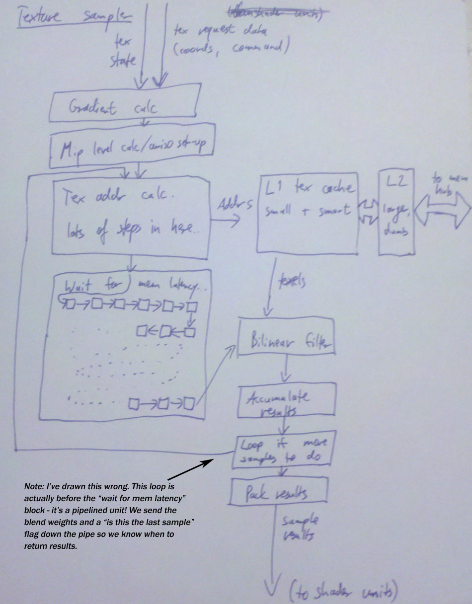