This post is part of the series “A trip through the Graphics Pipeline 2011”.
Not so fast.
In the previous part I explained the various stages that your 3D rendering commands go through on a PC before they actually get handed off to the GPU; short version: it’s more than you think. I then finished by name-dropping the command processor and how it actually finally does something with the command buffer we meticulously prepared. Well, how can I say this – I lied to you. We’ll indeed be meeting the command processor for the first time in this installment, but remember, all this command buffer stuff goes through memory – either system memory accessed via PCI Express, or local video memory. We’re going through the pipeline in order, so before we get to the command processor, let’s talk memory for a second.
The memory subsystem
GPUs don’t have your regular memory subsystem – it’s different from what you see in general-purpose CPUs or other hardware, because it’s designed for very different usage patterns. There’s two fundamental ways in which a GPU’s memory subsystem differs from what you see in a regular machine:
The first is that GPU memory subsystems are fast. Seriously fast. A Core i7 2600K will hit maybe 19 GB/s memory bandwidth – on a good day. With tail wind. Downhill. A GeForce GTX 480, on the other hand, has a total memory bandwidth of close to 180 GB/s – nearly an order of magnitude difference! Whoa.
The second is that GPU memory subsystems are slow. Seriously slow. A cache miss to main memory on a Nehalem (first-generation Core i7) takes about 140 cycles if you multiply the memory latency as given by AnandTech by the clock rate. The GeForce GTX 480 I mentioned previously has a memory access latency of 400-800 clocks. So let’s just say that, measured in cycles, the GeForce GTX 480 has a bit more than 4x the average memory latency of a Core i7. Except that Core i7 I just mentioned is clocked at 2.93GHz, whereas GTX 480 shader clock is 1.4 GHz – that’s it, another 2x right there. Woops – again, nearly an order of magnitude difference! Wait, something funny is going on here. My common sense is tingling. This must be one of those trade-offs I keep hearing about in the news!
Yep – GPUs get a massive increase in bandwidth, but they pay for it with a massive increase in latency (and, it turns out, a sizable hit in power draw too, but that’s beyond the scope of this article). This is part of a general pattern – GPUs are all about throughput over latency; don’t wait for results that aren’t there yet, do something else instead!
That’s almost all you need to know about GPU memory, except for one general DRAM tidbit that will be important later on: DRAM chips are organized as a 2D grid – both logically and physically. There’s (horizontal) row lines and (vertical) column lines. At each intersection between such lines is a transistor and a capacitor; if at this point you want to know how to actually build memory from these ingredients, Wikipedia is your friend. Anyway, the salient point here is that the address of a location in DRAM is split into a row address and a column address, and DRAM reads/writes internally always end up accessing all columns in the given row at the same time. What this means is that it’s much cheaper to access a swath of memory that maps to exactly one DRAM row than it is to access the same amount of memory spread across multiple rows. Right now this may seem like just a random bit of DRAM trivia, but this will become important later on; in other words, pay attention: this will be on the exam. But to tie this up with the figures in the previous paragraphs, just let me note that you can’t reach those peak memory bandwidth figures above by just reading a few bytes all over memory; if you want to saturate memory bandwidth, you better do it one full DRAM row at a time.
The PCIe host interface
From a graphics programmer standpoint, this piece of hardware isn’t super-interesting. Actually, the same probably goes for a GPU hardware architect too. The thing is, you still start caring about it once it’s so slow that it’s a bottleneck. So what you do is get good people on it to do it properly, to make sure that doesn’t happen. Other than that, well, this gives the CPU read/write access to video memory and a bunch of GPU registers, the GPU read/write access to (a portion of) main memory, and everyone a headache because the latency for all these transactions is even worse than memory latency because the signals have to go out of the chip, into the slot, travel a bit across the mainboard then get to someplace in the CPU about a week later (or that’s how it feels compared to the CPU/GPU speeds anyway). The bandwidth is decent though – up to about 8GB/s (theoretical) peak aggregate bandwidth across the 16-lane PCIe 2.0 connections that most GPUs use right now, so between half and a third of the aggregate CPU memory bandwidth; that’s a usable ratio. And unlike earlier standards like AGP, this is a symmetrical point-to-point link – that bandwidth goes both directions; AGP had a fast channel from the CPU to the GPU, but not the other way round.
Some final memory bits and pieces
Honestly, we’re very very close to actually seeing 3D commands now! So close you can almost taste them. But there’s one more thing we need to get out of the way first. Because now we have two kinds of memory – (local) video memory and mapped system memory. One is about a day’s worth of travel to the north, the other is a week’s journey to the south along the PCI Express highway. Which road do we pick?
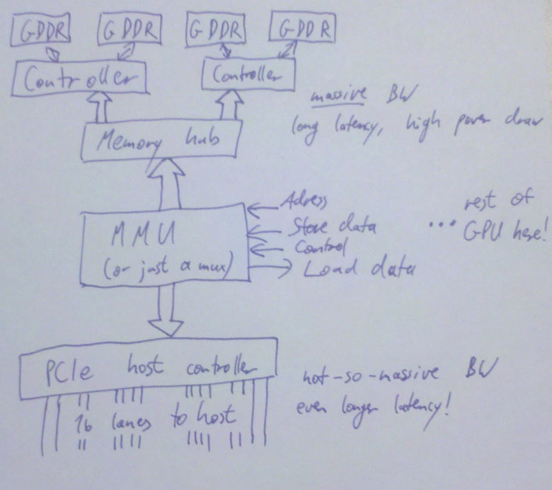
The easiest solution: Just add an extra address line that tells you which way to go. This is simple, works just fine and has been done plenty of times. Or maybe you’re on a unified memory architecture, like some game consoles (but not PCs). In that case, there’s no choice; there’s just the memory, which is where you go, period. If you want something fancier, you add a MMU (memory management unit), which gives you a fully virtualized address space and allows you to pull nice tricks like having frequently accessed parts of a texture in video memory (where they’re fast), some other parts in system memory, and most of it not mapped at all – to be conjured up from thing air, or, more usually, by a magic disk read that will only take about 50 years or so – and by the way, this is not hyperbole; if you stay with the “memory access = 1 day” metaphor, that’s really how long a single HD read takes. A quite fast one at that. Disks suck. But I digress.
So, MMU. It also allows you to defragment your video memory address space without having to actually copy stuff around when you start running out of video memory. Nice thing, that. And it makes it much easier to have multiple processes share the same GPU. It’s definitely allowed to have one, but I’m not actually sure if it’s a requirement or not, even though it’s certainly really nice to have (anyone care to help me out here? I’ll update the article if I get clarification on this, but tbh right now I just can’t be arsed to look it up). Anyway, a MMU/virtual memory is not really something you can just add on the side (not in an architecture with caches and memory consistency concerns anyway), but it really isn’t specific to any particular stage – I have to mention it somewhere, so I just put it here.
There’s also a DMA engine that can copy memory around without having to involve any of our precious 3D hardware/shader cores. Usually, this can at least copy between system memory and video memory (in both directions). It often can also copy from video memory to video memory (and if you have to do any VRAM defragmenting, this is a useful thing to have). It usually can’t do system memory to system memory copies, because this is a GPU, not a memory copying unit – do your system memory copies on the CPU where they don’t have to pass through PCIe in both directions!
Update: I’ve drawn a picture (link since this layout is too narrow to put big diagrams in the text). This also shows some more details – by now your GPU has multiple memory controllers, each of which controls multiple memory banks, with a fat hub in the front. Whatever it takes to get that bandwidth. :)
Okay, checklist. We have a command buffer prepared on the CPU. We have the PCIe host interface, so the CPU can actually tell us about this, and write its address to some register. We have the logic to turn that address into a load that will actually return data – if it’s from system memory it goes through PCIe, if we decide we’d rather have the command buffer in video memory, the KMD can set up a DMA transfer so neither the CPU nor the shader cores on the GPU need to actively worry about it. And then we can get the data from our copy in video memory through the memory subsystem. All paths accounted for, we’re set and finally ready to look at some commands!
At long last, the command processor!
Our discussion of the command processor starts, as so many things do these days, with a single word:
“Buffering…”
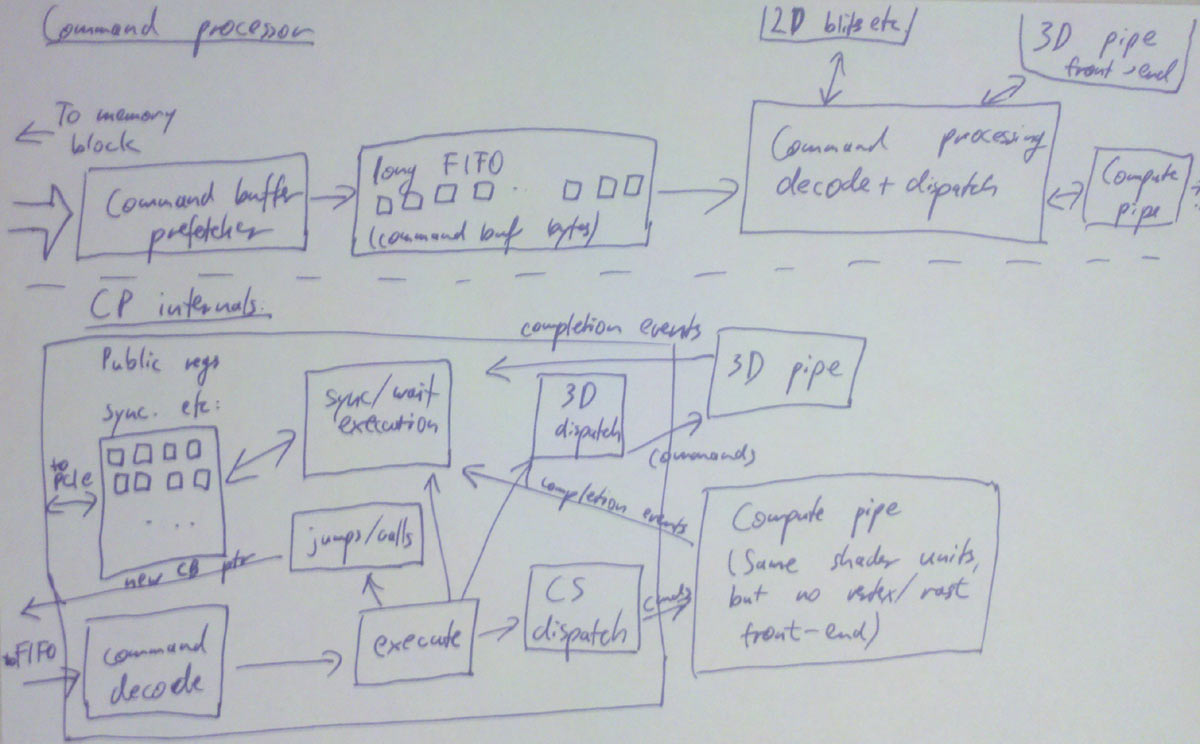
As mentioned above, both of our memory paths leading up to here are high-bandwidth but also high-latency. For most later bits in the GPU pipeline, the method of choice to work around this is to run lots of independent threads. But in this case, we only have a single command processor that needs to chew through our command buffer in order (since this command buffer contains things such as state changes and rendering commands that need to be executed in the right sequence). So we do the next best thing: Add a large enough buffer and prefetch far enough ahead to avoid hiccups.
From that buffer, it goes to the actual command processing front end, which is basically a state machine that knows how to parse commands (with a hardware-specific format). Some commands deal with 2D rendering operations – unless there’s a separate command processor for 2D stuff and the 3D frontend never even sees it. Either way, there’s still dedicated 2D hardware hidden on modern GPUs, just as there’s a VGA chip somewhere on that die that still supports text mode, 4-bit/pixel bit-plane modes, smooth scrolling and all that stuff. Good luck finding any of that on the die without a microscope. Anyway, that stuff exists, but henceforth I shall not mention it again. :) Then there’s commands that actually hand some primitives to the 3D/shader pipe, woo-hoo! I’ll take about them in upcoming parts. There’s also commands that go to the 3D/shader pipe but never render anything, for various reasons (and in various pipeline configurations); these are up even later.
Then there’s commands that change state. As a programmer, you think of them as just changing a variable, and that’s basically what happens. But a GPU is a massively parallel computer, and you can’t just change a global variable in a parallel system and hope that everything works out OK – if you can’t guarantee that everything will work by virtue of some invariant you’re enforcing, there’s a bug and you will hit it eventually. There’s several popular methods, and basically all chips use different methods for different types of state.
- Whenever you change a state, you require that all pending work that might refer to that state be finished (i.e. basically a partial pipeline flush). Historically, this is how graphics chips handled most state changes – it’s simple and not that costly if you have a low number of batches, few triangles and a short pipeline. Alas, batch and triangle counts have gone up and pipelines have gotten long, so the cost for this type of approach has shot up. It’s still alive and kicking for stuff that’s either changed infrequently (a dozen partial pipeline flushes aren’t that big a deal over the course of a whole frame) or just too expensive/difficult to implement with more specific schemes though.
- You can make hardware units completely stateless. Just pass the state change command through up to the stage that cares about it; then have that stage append the current state to everything it sends downstream, every cycle. It’s not stored anywhere – but it’s always around, so if some pipeline stage wants to look at a few bits in the state it can, because they’re passed in (and then passed on to the next stage). If your state happens to be just a few bits, this is fairly cheap and practical. If it happens to be the full set of active textures along with texture sampling state, not so much.
- Sometimes storing just one copy of the state and having to flush every time that stage changes serializes things too much, but things would really be fine if you had two copies (or maybe four?) so your state-setting frontend could get a bit ahead. Say you have enough registers (“slots”) to store two versions of every state, and some active job references slot 0. You can safely modify slot 1 without stopping that job, or otherwise interfering with it at all. Now you don’t need to send the whole state around through the pipeline – only a single bit per command that selects whether to use slot 0 or 1. Of course, if both slot 0 and 1 are busy by the time a state change command is encountered, you still have to wait, but you can get one step ahead. The same technique works with more than two slots.
- For some things like sampler or
textureShader Resource View state, you could be setting very large numbers of them at the same time, but chances are you aren’t. You don’t want to reserve state space for 2*128 active textures just because you’re keeping track of 2 in-flight state sets so you might need it. For such cases, you can use a kind of register renaming scheme – have a pool of 128 physical texture descriptors. If someone actually needs 128 textures in one shader, then state changes are gonna be slow. (Tough break). But in the more likely case of an app using less than 20 textures, you have quite some headroom to keep multiple versions around.
This is not meant to be a comprehensive list – but the main point is that something that looks as simple as changing a variable in your app (and even in the UMD/KMD and the command buffer for that matter!) might actually need a nontrivial amount of supporting hardware behind it just to prevent it from slowing things down.
Synchronization
Finally, the last family of commands deals with CPU/GPU and GPU/GPU synchronization.
Generally, all of these have the form “if event X happens, do Y”. I’ll deal with the “do Y” part first – there’s two sensible options for what Y can be here: it can be a push-model notification where the GPU yells at the CPU to do something right now (“Oi! CPU! I’m entering the vertical blanking interval on display 0 right now, so if you want to flip buffers without tearing, this would be the time to do it!”), or it can be a pull-model thing where the GPU just memorizes that something happened and the CPU can later ask about it (“Say, GPU, what was the most recent command buffer fragment you started processing?” – “Let me check… sequence id 303.”). The former is typically implemented using interrupts and only used for infrequent and high-priority events because interrupts are fairly expensive. All you need for the latter is some CPU-visible GPU registers and a way to write values into them from the command buffer once a certain event happens.
Say you have 16 such registers. Then you could assign currentCommandBufferSeqId to register 0. You assign a sequence number to every command buffer you submit to the GPU (this is in the KMD), and then at the start of each command buffer, you add a “If you get to this point in the command buffer, write to register 0”. And voila, now we know which command buffer the GPU is currently chewing on! And we know that the command processor finishes commands strictly in sequence, so if the first command in command buffer 303 was executed, that means all command buffers up to and including sequence id 302 are finished and can now be reclaimed by the KMD, freed, modified, or turned into a cheesy amusement park.
We also now have an example of what X could be: “if you get here” – perhaps the simplest example, but already useful. Other examples are “if all shaders have finished all texture reads coming from batches before this point in the command buffer” (this marks safe points to reclaim texture/render target memory), “if rendering to all active render targets/UAVs has completed” (this marks points at which you can actually safely use them as textures), “if all operations up to this point are fully completed”, and so on.
Such operations are usually called “fences”, by the way. There’s different methods of picking the values you write into the status registers, but as far as I am concerned, the only sane way to do it is to use a sequential counter for this (probably stealing some of the bits for other information). Yeah, I’m really just dropping that one piece of random information without any rationale whatsoever here, because I think you should know. I might elaborate on it in a later blog post (though not in this series) :).
So, we got one half of it – we can now report status back from the GPU to the CPU, which allows us to do sane memory management in our drivers (notably, we can now find out when it’s safe to actually reclaim memory used for vertex buffers, command buffers, textures and other resources). But that’s not all of it – there’s a puzzle piece missing. What if we need to synchronize purely on the GPU side, for example? Let’s go back to the render target example. We can’t use that as a texture until the rendering is actually finished (and some other steps have taken place – more details on that once I get to the texturing units). The solution is a “wait”-style instruction: “Wait until register M contains value N”. This can either be a compare for equality, or less-than (note you need to deal with wraparounds here!), or more fancy stuff – I’m just going with equals for simplicity. This allows us to do the render target sync before we submit a batch. It also allows us to build a full GPU flush operation: “Set register 0 to ++seqId if all pending jobs finished” / “Wait until register 0 contains seqId”. Done and done. GPU/GPU synchronization: solved – and until the introduction of DX11 with Compute Shaders that have another type of more fine-grained synchronization, this was usually the only synchronization mechanism you had on the GPU side. For regular rendering, you simply don’t need more.
By the way, if you can write these registers from the CPU side, you can use this the other way too – submit a partial command buffer including a wait for a particular value, and then change the register from the CPU instead of the GPU. This kind of thing can be used to implement D3D11-style multithreaded rendering where you can submit a batch that references vertex/index buffers that are still locked on the CPU side (probably being written to by another thread). You simply stuff the wait just in front of the actual render call, and then the CPU can change the contents of the register once the vertex/index buffers are actually unlocked. If the GPU never got that far in the command buffer, the wait is now a no-op; if it did, it spend some (command processor) time spinning until the data was actually there. Pretty nifty, no? Actually, you can implement this kind of thing even without CPU-writeable status registers if you can modify the command buffer after you submit it, as long as there’s a command buffer “jump” instruction. The details are left to the interested reader :)
Of course, you don’t necessarily need the set register/wait register model; for GPU/GPU synchronization, you can just as simply have a “rendertarget barrier” instruction that makes sure a rendertarget is safe to use, and a “flush everything” command. But I like the set register-style model more because it kills two birds (back-reporting of in-use resources to the CPU, and GPU self-synchronization) with one well-designed stone.
Update: Here, I’ve drawn a diagram for you. It got a bit convoluted so I’m going to lower the amount of detail in the future. The basic idea is this: The command processor has a FIFO in front, then the command decode logic, execution is handled by various blocks that communicate with the 2D unit, 3D front-end (regular 3D rendering) or shader units directly (compute shaders), then there’s a block that deals with sync/wait commands (which has the publicly visible registers I talked about), and one unit that handles command buffer jumps/calls (which changes the current fetch address that goes to the FIFO). And all of the units we dispatch work to need to send us back completion events so we know when e.g. textures aren’t being used anymore and their memory can be reclaimed.
Closing remarks
Next step down is the first one doing any actual rendering work. Finally, only 3 parts into my series on GPUs, we actually start looking at some vertex data! (No, no triangles being rasterized yet. That will take some more time).
Actually, at this stage, there’s already a fork in the pipeline; if we’re running compute shaders, the next step would already be … running compute shaders. But we aren’t, because compute shaders are a topic for later parts! Regular rendering pipeline first.
Small disclaimer: Again, I’m giving you the broad strokes here, going into details where it’s necessary (or interesting), but trust me, there’s a lot of stuff that I dropped for convenience (and ease of understanding). That said, I don’t think I left out anything really important. And of course I might’ve gotten some things wrong. If you find any bugs, tell me!
Until the next part…
This post is part of the series “A trip through the Graphics Pipeline 2011”.
It’s been awhile since I posted something here, and I figured I might use this spot to explain some general points about graphics hardware and software as of 2011; you can find functional descriptions of what the graphics stack in your PC does, but usually not the “how” or “why”; I’ll try to fill in the blanks without getting too specific about any particular piece of hardware. I’m going to be mostly talking about DX11-class hardware running D3D9/10/11 on Windows, because that happens to be the (PC) stack I’m most familiar with – not that the API details etc. will matter much past this first part; once we’re actually on the GPU it’s all native commands.
The application
This is your code. These are also your bugs. Really. Yes, the API runtime and the driver have bugs, but this is not one of them. Now go fix it already.
The API runtime
You make your resource creation / state setting / draw calls to the API. The API runtime keeps track of the current state your app has set, validates parameters and does other error and consistency checking, manages user-visible resources, may or may not validate shader code and shader linkage (or at least D3D does, in OpenGL this is handled at the driver level) maybe batches work some more, and then hands it all over to the graphics driver – more precisely, the user-mode driver.
The user-mode graphics driver (or UMD)
This is where most of the “magic” on the CPU side happens. If your app crashes because of some API call you did, it will usually be in here :). It’s called “nvd3dum.dll” (NVidia) or “atiumd*.dll” (AMD). As the name suggests, this is user-mode code; it’s running in the same context and address space as your app (and the API runtime) and has no elevated privileges whatsoever. It implements a lower-level API (the DDI) that is called by D3D; this API is fairly similar to the one you’re seeing on the surface, but a bit more explicit about things like memory management and such.
This module is where things like shader compilation happen. D3D passes a pre-validated shader token stream to the UMD – i.e. it’s already checked that the code is valid in the sense of being syntactically correct and obeying D3D constraints (using the right types, not using more textures/samplers than available, not exceeding the number of available constant buffers, stuff like that). This is compiled from HLSL code and usually has quite a number of high-level optimizations (various loop optimizations, dead-code elimination, constant propagation, predicating ifs etc.) applied to it – this is good news since it means the driver benefits from all these relatively costly optimizations that have been performed at compile time. However, it also has a bunch of lower-level optimizations (such as register allocation and loop unrolling) applied that drivers would rather do themselves; long story short, this usually just gets immediately turned into a intermediate representation (IR) and then compiled some more; shader hardware is close enough to D3D bytecode that compilation doesn’t need to work wonders to give good results (and the HLSL compiler having done some of the high-yield and high-cost optimizations already definitely helps), but there’s still lots of low-level details (such as HW resource limits and scheduling constraints) that D3D neither knows nor cares about, so this is not a trivial process.
And of course, if your app is a well-known game, programmers at NV/AMD have probably looked at your shaders and wrote hand-optimized replacements for their hardware – though they better produce the same results lest there be a scandal :). These shaders get detected and substituted by the UMD too. You’re welcome.
More fun: Some of the API state may actually end up being compiled into the shader – to give an example, relatively exotic (or at least infrequently used) features such as texture borders are probably not implemented in the texture sampler, but emulated with extra code in the shader (or just not supported at all). This means that there’s sometimes multiple versions of the same shader floating around, for different combinations of API states.
Incidentally, this is also the reason why you’ll often see a delay the first time you use a new shader or resource; a lot of the creation/compilation work is deferred by the driver and only executed when it’s actually necessary (you wouldn’t believe how much unused crap some apps create!). Graphics programmers know the other side of the story – if you want to make sure something is actually created (as opposed to just having memory reserved), you need to issue a dummy draw call that uses it to “warm it up”. Ugly and annoying, but this has been the case since I first started using 3D hardware in 1999 – meaning, it’s pretty much a fact of life by this point, so get used to it. :)
Anyway, moving on. The UMD also gets to deal with fun stuff like all the D3D9 “legacy” shader versions and the fixed function pipeline – yes, all of that will get faithfully passed through by D3D. The 3.0 shader profile ain’t that bad (it’s quite reasonable in fact), but 2.0 is crufty and the various 1.x shader versions are seriously whack – remember 1.3 pixel shaders? Or, for that matter, the fixed-function vertex pipeline with vertex lighting and such? Yeah, support for all that’s still there in D3D and the guts of every modern graphics driver, though of course they just translate it to newer shader versions by now (and have been doing so for quite some time).
Then there’s things like memory management. The UMD will get things like texture creation commands and need to provide space for them. Actually, the UMD just suballocates some larger memory blocks it gets from the KMD (kernel-mode driver); actually mapping and unmapping pages (and managing which part of video memory the UMD can see, and conversely which parts of system memory the GPU may access) is a kernel-mode privilege and can’t be done by the UMD.
But the UMD can do things like swizzling textures (unless the GPU can do this in hardware, usually using 2D blitting units not the real 3D pipeline) and schedule transfers between system memory and (mapped) video memory and the like. Most importantly, it can also write command buffers (or “DMA buffers” – I’ll be using these two names interchangeably) once the KMD has allocated them and handed them over. A command buffer contains, well, commands :). All your state-changing and drawing operations will be converted by the UMD into commands that the hardware understands. As will a lot of things you don’t trigger manually – such as uploading textures and shaders to video memory.
In general, drivers will try to put as much of the actual processing into the UMD as possible; the UMD is user-mode code, so anything that runs in it doesn’t need any costly kernel-mode transitions, it can freely allocate memory, farm work out to multiple threads, and so on – it’s just a regular DLL (even though it’s loaded by the API, not directly by your app). This has advantages for driver development too – if the UMD crashes, the app crashes with it, but not the whole system; it can just be replaced while the system is running (it’s just a DLL!); it can be debugged with a regular debugger; and so on. So it’s not only efficient, it’s also convenient.
But there’s a big elephant in the room that I haven’t mentioned yet.
Did I say “user-mode driver”? I meant “user-mode drivers”.
As said, the UMD is just a DLL. Okay, one that happens to have the blessing of D3D and a direct pipe to the KMD, but it’s still a regular DLL, and in runs in the address space of its calling process.
But we’re using multi-tasking OSes nowadays. In fact, we have been for some time.
This “GPU” thing I keep talking about? That’s a shared resource. There’s only one that drives your main display (even if you use SLI/Crossfire). Yet we have multiple apps that try to access it (and pretend they’re the only ones doing it). This doesn’t just work automatically; back in The Olden Days, the solution was to only give 3D to one app at a time, and while that app was active, all others wouldn’t have access. But that doesn’t really cut it if you’re trying to have your windowing system use the GPU for rendering. Which is why you need some component that arbitrates access to the GPU and allocates time-slices and such.
Enter the scheduler.
This is a system component – note the “the” is somewhat misleading; I’m talking about the graphics scheduler here, not the CPU or IO schedulers. This does exactly what you think it does – it arbitrates access to the 3D pipeline by time-slicing it between different apps that want to use it. A context switch incurs, at the very least, some state switching on the GPU (which generates extra commands for the command buffer) and possibly also swapping some resources in and out of video memory. And of course only one process gets to actually submit commands to the 3D pipe at any given time.
You’ll often find console programmers complaining about the fairly high-level, hands-off nature of PC 3D APIs, and the performance cost this incurs. But the thing is that 3D APIs/drivers on PC really have a more complex problem to solve than console games – they really do need to keep track of the full current state for example, since someone may pull the metaphorical rug from under them at any moment! They also work around broken apps and try to fix performance problems behind their backs; this is a rather annoying practice that no-one’s happy with, certainly including the driver authors themselves, but the fact is that the business perspective wins here; people expect stuff that runs to continue running (and doing so smoothly). You just won’t win any friends by yelling “BUT IT’S WRONG!” at the app and then sulking and going through an ultra-slow path.
Anyway, on with the pipeline. Next stop: Kernel mode!
The kernel-mode driver (KMD)
This is the part that actually deals with the hardware. There may be multiple UMD instances running at any one time, but there’s only ever one KMD, and if that crashes, then boom you’re dead – used to be “blue screen” dead, but by now Windows actually knows how to kill a crashed driver and reload it (progress!). As long as it happens to be just a crash and not some kernel memory corruption at least – if that happens, all bets are off.
The KMD deals with all the things that are just there once. There’s only one GPU memory, even though there’s multiple apps fighting over it. Someone needs to call the shots and actually allocate (and map) physical memory. Similarly, someone must initialize the GPU at startup, set display modes (and get mode information from displays), manage the hardware mouse cursor (yes, there’s HW handling for this, and yes, you really only get one! :), program the HW watchdog timer so the GPU gets reset if it stays unresponsive for a certain time, respond to interrupts, and so on. This is what the KMD does.
There’s also this whole content protection/DRM bit about setting up a protected/DRM’ed path between a video player and the GPU so no the actual precious decoded video pixels aren’t visible to any dirty user-mode code that might do awful forbidden things like dump them to disk (…whatever). The KMD has some involvement in that too.
Most importantly for us, the KMD manages the actual command buffer. You know, the one that the hardware actually consumes. The command buffers that the UMD produces aren’t the real deal – as a matter of fact, they’re just random slices of GPU-addressable memory. What actually happens with them is that the UMD finishes them, submits them to the scheduler, which then waits until that process is up and then passes the UMD command buffer on to the KMD. The KMD then writes a call to command buffer into the main command buffer, and depending on whether the GPU command processor can read from main memory or not, it may also need to DMA it to video memory first. The main command buffer is usually a (quite small) ring buffer – the only thing that ever gets written there is system/initialization commands and calls to the “real”, meaty 3D command buffers.
But this is still just a buffer in memory right now. Its position is known to the graphics card – there’s usually a read pointer, which is where the GPU is in the main command buffer, and a write pointer, which is how far the KMD has written the buffer yet (or more precisely, how far it has told the GPU it has written yet). These are hardware registers, and they are memory-mapped – the KMD updates them periodically (usually whenever it submits a new chunk of work)…
The bus
…but of course that write doesn’t go directly to the graphics card (at least unless it’s integrated on the CPU die!), since it needs to go through the bus first – usually PCI Express these days. DMA transfers etc. take the same route. This doesn’t take very long, but it’s yet another stage in our journey. Until finally…
The command processor!
This is the frontend of the GPU – the part that actually reads the commands the KMD writes. I’ll continue from here in the next installment, since this post is long enough already :)
Small aside: OpenGL
OpenGL is fairly similar to what I just described, except there’s not as sharp a distinction between the API and UMD layer. And unlike D3D, the (GLSL) shader compilation is not handled by the API at all, it’s all done by the driver. An unfortunate side effect is that there are as many GLSL frontends as there are 3D hardware vendors, all of them basically implementing the same spec, but with their own bugs and idiosyncrasies. Not fun. And it also means that the drivers have to do all the optimizations themselves whenever they get to see the shaders – including expensive optimizations. The D3D bytecode format is really a cleaner solution for this problem – there’s only one compiler (so no slightly incompatible dialects between different vendors!) and it allows for some costlier data-flow analysis than you would normally do.
Omissions and simplifcations
This is just an overview; there’s tons of subtleties that I glossed over. For example, there’s not just one scheduler, there’s multiple implementations (the driver can choose); there’s the whole issue of how synchronization between CPU and GPU is handled that I didn’t explain at all so far. And so on. And I might have forgotten something important – if so, please tell me and I’ll fix it! But now, bye and hopefully see you next time.
There’s two major (no pun intended) ways to store 2D arrays: Row-major and Column-major. Row-major is the default layout in C, Pascal and most other programming languages; column-major is the default in FORTRAN and some numeric math-centric languages (mainly Matlab and R) – presumably because they started out as a kind of frontend for FORTRAN code.
Confusingly, the same terminology is also used by some people to denote whether you’re treating vectors as column vectors or row vectors by default. If you treat them as column vectors, you typically multiply a vector with a matrix from the left, i.e. the result of transforming a vector v by a matrix M is written 


Historically, IRIS GL used the row-vector convention, then OpenGL (which was based on IRIS GL) switched to column vectors in its specification (to make it match up better with standard mathematical practice) but at the same time switched storage layout from row-major to column-major to make sure that existing IRIS GL code didn’t break. That’s a somewhat unfortunate legacy, since C defaults to row-major storage, so you would normally expect a C library to use that too. ES got rid of a lot of other historical ballast, so this would’ve been a good place to change it.
Anyway, a priori, there’s no huge reason to strongly prefer one storage layout over the other. However in some cases, external constraints tilt the balance. I recently bitched a bit about OpenGL ES favoring column-major order, because it happens to be such a case, and column-major is the wrong choice. Don’t get me wrong, it’s by no means a big deal anyway, but it makes things less orthogonal than they need to be, which annoys me.
GLSL and HLSL have vec4/float4 as their basic native vector data type, and shader constants are usually passed in groups of 4 floats (as of D3D10+ HW this is a bit more freeform, but the alignment/packing rules are still float4-centric). In a row-major layout, a 4×4 matrix gets stored as
struct mat4_row_major {
  vec4 row0;
  vec4 row1;
  vec4 row2;
  vec4 row3;
};
and multiplying a matrix with a 4-vector gets computed as
  // This implements o = M*v
  o.x = dot(M.row0, v);
  o.y = dot(M.row1, v);
  o.z = dot(M.row2, v);
  o.w = dot(M.row3, v);
whereas for column-major storage layout you get
struct mat4_col_major {
  vec4 col0;
  vec4 col1;
  vec4 col2;
  vec4 col3;
};

  // M*v expands to...
  o = M.col0 * v.x;
  o += M.col1 * v.y;
  o += M.col2 * v.z;
  o += M.col3 * v.w;
so column-major uses muls/multiply-adds whereas row-major storage ends up using dot products. Same difference, so far – generally, shaders take the exact same time for both variants. But there’s an important special case: affine transforms, i.e. ones for which the last row of the matrix is “0 0 0 1”. Generally almost all of the transforms you’ll use in a game/rendering engine, except for the final projection transform, are of this form. More concretely, all of the transforms you’ll normally use for character skinning are affine, and if you do skinning in a shader you’ll use a lot of them, so their size matters. With the row-major layout you can just drop the last row and do this:
  // M*v, where M is affine with last row not stored
  o.x = dot(M.row0, v);
  o.y = dot(M.row1, v);
  o.z = dot(M.row2, v);
  o.w = v.w; // often v.w==1 so this simplifies further
while with the column-major layout, you get to drop the last entry of every column vector, but that saves neither memory nor shader instructions. (As an aside, GL ES doesn’t support non-square matrix types directly; if you want to use a non-square matrix, you have to use an array/struct of vecs instead – another annoyance)
Furthermore, I generally prefer (for rendering code anyway) to store matrices in the format that I’m gonna send to the hardware or graphics API. On GL ES, that means I have to do one of three things:
- Use 4×4 matrices everywhere and live with 25% unnecessary extra arithmetic and memory transfers,
- Have my 3×4 matrix manipulation use row-major layout while 4×4 uses column-major,
- Avoid the GL ES builtin mat4 type and use a vec4[4] (or a corresponding struct) instead.
Now, options 2 and 3 are perfectly workable, but they’re ugly, and it annoys me that an API that breaks compatibility with the original OpenGL in about 50 different ways anyway didn’t clean up this historical artifact.
This is a bit unsorted – just a bunch of things I wanted to write down at some point but didn’t feel like writing a full article about.
Cache size is measured in lines, not bytes
This is important to keep in mind when thinking about cache utilization, particularly L1. For example, the Cell (and also the Xbox 360 CPU) has 32k of L1 data cache but 128-byte cache lines, i.e. 256 cache lines total. Compare to e.g. the original 1993 Intel Pentium, which has 8k of L1 and 32-byte cache lines, for a total of… 256 cache lines! If your data is laid out sequentially, you get to use the 4x increased capacity. But when you use linked data structures, you really don’t: you’re more likely than not to end up in a different cache line every time you dereference a pointer, so assuming each node fits into a cache line, you’re limited to 256 nodes in your L1. Tops. Assuming no node straddles two cache lines and there are no set conflicts whatsoever.
32k of cache may sound like enough to keep your hot data structures in them – but if you use linked data structures with small nodes, you only really get to use a fraction. Good thing to keep in mind.
“Hardware thread” is an awful name
It just is. Overloading the term “thread” is a poor choice – when talking among software people anyway. When talking about code running on chips with SMT (Simultaneous multithreading, aka “HyperThreading” in Intel parlance) there’s instant confusion whenever the word “thread” is used, since it could either be a “software” (OS) thread or a hardware one.
Make up your own terminology, goddamnit! “Threads” (like “Processes”, “Fibers” and “Files”) are a software concept – an abstraction provided by the OS. A hardware thread isn’t a thread at all; it’s some extra infrastructure added to the hardware that is typically used by the OS to implement the “thread” abstraction. It deserves its own name.
That said, I don’t have any brilliant suggestions either. The best I’ve come up with so far is “head”, which is just a portmanteau of “Hardware thread” into a nice pronunciation-friendly one-syllable word. Pros are that it’s from a semantic field not yet overused in programming (body parts), and it suggests a nice metaphor: imagine a hydra which has multiple heads but just one torso – that’s roughly how SMT processors work. Cons are that it’s not really catchy and phonetically too similar to “thread”. As said, it’s not perfect. I’d be glad to hear better suggestions!
And while we’re on the subject of terminology, I submit this for your consideration: Just continue the list from Fiber->Thread naturally! A thread group is a “rope”, and a group of ropes (thread groups) is a “dew”. Yes, it’s only half-serious, but with the 3-dimensional D3D11 compute shader “thread coordinates” it doesn’t seem that silly anymore…
Hardware threads compete for core resources!
Remember those 256 cache lines up there? Yeah, that’s if you’re only using one head. If you’re using two, they’re both running out of the same L1 cache, and neither will get all 256 lines – with fun interference all around. The same goes for instruction cache, by the way. A great way to get 2-way hardware multithreading except-not-really is by running 2 threads with code that branches around a lot. Pick your poison: use large unrolled functions with plenty of inlining and run out of L1 I$ capacity, or use lots of small functions with tons of calls and end up using I$ lines inefficiently (and eating lots of branch penalties besides). The only winning move is not to play that game in the first place. What you want is reasonably small, tight loops. Especially if you’re using multiple HW threads – since you usually also only get half the branch prediction slots, half the BTB entries, and so on.
Also note that extra heads really aren’t like extra cores. If you have more cores, you can get substantial speedups even using algorithms that don’t scale linearly (i.e. more threads cause some amount of extra work). With extra heads, that doesn’t work, or at least doesn’t work very well; if you’re running into a bottleneck of the core (be it computation, memory bandwidth, instruction decoding, or something else), adding extra heads doesn’t help – they’re meant to avoid stalls. If you’re keeping the core busy as-is, you need an extra head about as much as you… well, need a second head, actually. :) And there’s also the bit about the smaller effective data cache size and so on. Of course there’s advantages too: heads on one core can share data much more efficiently than different cores can since they’re using the same L1 cache, they have no coherency traffic between them, and they don’t suffer from false sharing. So they’re very well suited to low-latency fine-grained threading.
Threads, threads, and threads
The concept of threads (the software kind) has been around for a while, but not all threads are created (or should I say designed?) equal. Threads are used for different reasons, and even some fit the underlying OS thread abstraction better than others.
The first major use case is different “subprograms” that execute concurrently from the user’s point of view – the OS might decide to put two threads onto different cores so they actually execute at the same time, or it might opt to multiplex both onto one core by time-slicing. This is the “original” thread model; it’s what you use to keep UI responsive even when the app is doing some intensive number crunching right now, etc. It’s what OSes expect you to do when you create a thread.
The second case is where you want the different “subprograms”, but not the concurrency. You use threads purely to have several execution contexts in your program, but they don’t run simultaneously, and you “switch” from one to the other at set points (by “starting” thread 2 and putting thread 1 to sleep by waiting on some event/condition variable). Basically, all you want from threads is to have two separate stacks. This is effectively using OS facilities to implement coroutines in a language that doesn’t have them. Of course, this is overkill – threads are fairly heavyweight entities and they get scheduled; that’s a big price to pay for what’s effectively a stack-switching mechanism. When OS developers saw people doing this, they introduced “Fibers” to fill the niche. These exist (under different names) in basically all modern OSes and allow you to have multiple stacks, program counters and hence flows of execution, but without preemption and most of the hidden costs involved in creating a thread.
The third case is threads you create exclusively for the purpose of getting concurrency, i.e. what’s commonly called “worker threads”. Unlike the first two groups, they typically all run the same code (or at least the same main loop). This only makes sense if you have multiple cores, or one core with SMT. If you have neither, cut out the middleman – just process the work in your main thread! Anyway, this kind of thread has existed for a long time in the server and high-performance computing world, but its appearance on the desktop is relatively recent. And it shows: OSes don’t have really great support for this kind of thread yet. There’s lot of support code and libraries, but worker threads aren’t really first-class citizens at the OS level yet.
There’s two problems: First, the way this is currently done is by setting up a “thread pool”. At startup time, you create some number of threads (usually as many as the number of available “logical” processors minus 1 for the main thread) to be worker threads. The threads all check if there’s work queued up, execute it if available and go to sleep if there’s nothing to do. This works fine if all threads actually get assigned to a different head, but it quickly starts to suck once there’s other apps doing the same thing, especially if one or more of them mess around with thread or process affinities. The second, more serious problem affects latency-critical applications, which on desktop OSes usually means soft real-time apps like games or media players. Such programs usually work frame-based, with one sync-point per frame where results must be ready (not necessarily results from a computation started this frame – the process can be pipelined across more than one frame – but the “one sync per frame” design is fairly common). This design interacts really badly with OS context switches. Here’s a simple example with 16 jobs distributed across 4 worker threads to illustrate the problem:

Worker 3 gets interrupted shortly after it grabs its fourth job, and before it finishes. At that point in time, there’s three remaining tasks left, which the three other workers divide among each other. And then the task list is empty and everyone waits for Worker 3 to finish… and waits… and waits some more until Worker 3 finally gets re-activated and finishes its job. Ouch – it would’ve been much faster if Worker 3 had only processed 3 items then gone to sleep, with the remaining 3 threads dividing up 4 jobs.
It all depends on timing. If you have a system that’s self-balancing (e.g. a “work stealing” type job manager), you will avoid most of the extra cost when one of the workers is interrupted early in the frame: the remaining threads just crunch through the work alone while one thread stalls. But if the interruption is shortly before a sync point, you’re just screwed no matter what you do.
This is really a scheduling problem. If you have a worker thread, it’s great to interrupt them when they’ve just finished a job, and extremely bad to interrupt them just after they agreed to start work on a new one. Ideally, you’d have a semi-cooperative multitasking system for worker threads; after every job (or every 10 jobs or whatever, depending on granularity), worker threads do a syscall that signals “if you want to do a context switch, now would be a good time”. This is not the same as a “sleep”/”yield” type operation; we don’t want to relinquish our time slice, just signal that now is a good time to schedule something different if the time is almost up! The scheduler in turn promises to only do context switches at these points, unless it hasn’t seen one in some set time interval (say 20ms or so), after which the thread is up for regular preemption.
That’s a quick patch, but really you want to make the OS to be aware of worker threads on a deep level, just as it “knows” Threads and Fibers right now. A static thread pool works fine if you have exclusive control of the system, but it’s the wrong model for a desktop OS. If you have multiple apps each running their own thread pools, you don’t want to multiplex them onto the available hardware threads; ideally you want to change the number of worker threads available to each app instead! But to do this properly, the OS needs to be aware of the distinction first.
This is gonna be a short one. Let’s start with this simple loop to compute the dot product of two vectors vec_a, vec_b of signed 16-bit values:
	; (rsi=vec_a, rdi=vec_b, rcx=N_elements/16)
	pxor		xmm0, xmm0
	pxor		xmm1, xmm1

dot_loop:
	movdqa		xmm2, [rsi]
	movdqa		xmm3, [rsi+16]
	pmaddwd		xmm2, [rdi]
	pmaddwd		xmm3, [rdi+16]
	paddd		xmm0, xmm2
	paddd		xmm1, xmm3
	add		rsi, 32
	add		rdi, 32
	dec		rcx
	jnz		dot_loop
There’s nothing really wrong with this code, but it executes more ops per loop iteration than strictly necessary. Whether this actually costs you cycles (and how many) heavily depends on the processor you’re running on, so I’ll dodge that subject for a bit and pretend there’s no out-of-order execution to help us and every instruction costs at least one cycle.
Anyway, the key insight here is that we’re basically using three registers (rsi, rdi, rcx) as counters, and we end up updating all of them. The key is to update less counters and shift some of the work to the magic x86 addressing modes. One way to do this is to realize that while rsi and rdi change every iteration, rdi - rsi is loop invariant. So we can compute it once and do this:
	sub		rdi, rsi
	pxor		xmm0, xmm0
	pxor		xmm1, xmm1

some_loop:
	movdqa		xmm2, [rsi]
	movdqa		xmm3, [rsi+16]
	pmaddwd		xmm2, [rsi+rdi]
	pmaddwd		xmm3, [rsi+rdi+16]
	paddd		xmm0, xmm2
	paddd		xmm1, xmm3
	add		rsi, 32
	dec		rcx
	jnz		some_loop
One sub extra before the loop, but one less add inside the loop (of course we do that work in the addressing modes now, but luckily for us, they’re basically free).
There’s a variant of this that computes vec_a_end = rsi + rcx*32 at the start and replaces the dec rcx with a cmp rsi, vec_a_end. Two more instructions at the loop head, no instructions saved inside the loop, but we get a cmp/jne pair which Core2 onwards can fuse into one micro-op, so that’s a plus. VC++ will often generate this style of code for simple loops.
We can still go one lower, though – there’s still two adds (or one add+one compare), after all! The trick is to use a loop count in bytes instead of elements and have it count up from -sizeof(vec_a) to zero, so we can still use one jnz at the end to do our conditional jump. The code looks like this:
	shl		rcx, 5			; sizeof(vec_a)
	pxor		xmm0, xmm0
	pxor		xmm1, xmm1
	add		rsi, rcx		; end of vec_a
	add		rdi, rcx		; end of vec_b
	neg		rcx

some_loop:
	movdqa		xmm2, [rsi+rcx]
	movdqa		xmm3, [rsi+rcx+16]
	pmaddwd		xmm2, [rdi+rcx]
	pmaddwd		xmm3, [rdi+rcx+16]
	paddd		xmm0, xmm2
	paddd		xmm1, xmm3
	add		rcx, 32
	jnz		some_loop
The trend should be clear at this point – a few more instrs in the loop head, but less work inside the loop. How much less depends on the processor. But the newest batch of Core i7s (Sandy Bridge) can fuse the add/jnz pair into one micro-op, so it’s very cheap indeed.
This is about the “secret ingredient” in my EXE packer kkrunchy, which was used in our (Farbrausch) 64k intros starting from “fr-030: Candytron”, and also in a lot of other 64k intros or similarly size-limited productions by other groups – including several well-known 64ks from other groups such as Conspiracy, Equinox and Fairlight, I’m happy to add.
There are two primary versions of kkrunchy. The first one was developed between 2003 and 2005 and uses a fairly simple LZ77 coder with arithmetic coding backend, designed to have good compression and a small depacker (about 300 bytes when using hand-optimized x86 code). If you’re interested in the details, a simplified C++ version of the depacker that I then used to write the ASM code from is still available here (of the various programs I’ve written, this is still one of my favorites: it’s just nice to have something so fundamentally simple that’s actually useful).
The second was developed roughly between 2006 and 2008 and uses PAQ-style context mixing. To be precise, it’s a spin-off borrowing a lot of ideas from PAQ7 including its neural network mixer, but with a custom model design optimized to use a lot less memory (around 5.5mb instead of hundreds of megabytes) and run a lot faster. It’s still dog slow, but it managed to process >120kb/s on my then-current P4 2.4GHz instead of the roughly 5kb/s that PAQ7 managed on the same machine when targeting roughly the same compression ratio. The depacker was optimized for both size and speed (with this much computation per bit, making it 4x slower for the sake of saving a few bytes is a bad deal!), and took up a comparatively hefty 1.5k, but normally more than made up for it. For example, our 96k shooter “kkrieger” shrunk by over 10k when recompressed with the new engine (if only we’d had that before, it would’ve saved us a lot of work in the last week before release and prevented some very embarrassing bugs).
Anyway, both packing engines were competitive with the state of the art in EXE compression for the given target sizes when they were first released, but neither were in any way spectacular, and both were biased towards simplicity and tweakability, not absolutely maximum compression. That’s because unlike most other EXE packers, kkrunchy doesn’t rely solely on its backend compression engine to bring in the space savings.
This is a small one, for all compression geeks out there.
The Elias gamma code (closely related to Exponential-Golomb codes, or Exp-Golomb codes for short) is very useful for practical compression applications; it certainly crops up in a lot of modern video coding standards, for example. The mapping goes like this:
  1 -> 1
  2 -> 010
  3 -> 011
  4 -> 00100
  5 -> 00101
  6 -> 00110
  7 -> 00111
  8 -> 0001000
and so on (Exp-Golomb with k=0 is the same, except the first index encoded is 0 not 1, i.e. there’s an implicit added 1 during encoding and a subtracted 1 during decoding).
Anyway, if you want to decode this quickly, and if your bit buffer reads bits from the MSB downwards, shifting after every read so the first unconsumed bit is indeed the MSB (there’s very good reasons for doing it this way; I might blog about this at some point), then there’s a very nifty way to decode this quickly:
  // at least one of the top 12 bits set?
  // (this means less than 12 heading zeros)
  if (bitbuffer & (~0u << (32 - 12))) {
    // this is the FAST path
    U32 num_zeros = CountLeadingZeros(bitbuffer);
    return GetBits(num_zeros * 2 + 1);
  } else {
    // coded value is longer than 25 bits, need to
    // use slow path (read however you would read
    // gamma codes regularly)
  }
Note that this is one CountLeadingZeros and one GetBits operation. The GetBits reads both the zeros and the actual value in one go; it just so happens that the binary value of that is exactly the value we need to decode. Not earth-shaking, but nice to know. In practice, it means you can read such codes very quickly indeed (it’s just a handful of opcodes on both x86 with bsr and PowerPC with cntlzw or cntlzd if you’re using a 64-bit buffer).
This is assuming a 32-bit shift register that contains your unread bits, refilled by reading another byte whenever there’s 24 or less unconsumed bits available (a fairly typical choice). If you have 64-bit registers, it’s usually better to keep a 64-bit buffer and refill whenever the available number of bits is 32 or less. In that case you can read gamma codes of up to 33 bits length (i.e. 16 heading 0 bits) directly.
If you’re working with images in your program, you’re most likely using a regular 2D array layout to store image data. Which is to say, it’s basically a 1D array of width * height pixels, and the index of every pixel in the array is normally computed as y * width + x (or, more generally, y * stride + x when you don’t require the lines to be densely packed). Simple and easy, but it has a problem: if you have a cache, this is very efficient when processing pixels in one direction (left to right) and very inefficient if you move at a 90 degree angle to that direction (top to bottom): the first pixel of every row is in a different cache line (unless your image is tiny), so you get tons of cache misses.
That’s one of the reasons why GPUs tend to prefer tiled or swizzled texture formats, which depart from the purely linear memory layout to something a tad more involved. The specifics heavily depend on the internals of the memory subsystem, but while the respective magic values may be different between different pieces of hardware, the general principles are always the same.
The data structure is extremely simple: a bounded FIFO. One step up from plain arrays, but still, it’s very basic stuff. And if you’re doing system programming, particularly anything involving IO or directly talking to hardware (boils down to the same thing really), it’s absolutely everywhere. It’s also very useful to communicate between different threads. I have some notes on the topic than aren’t immediately obvious, so it’s time to write them up. I’m only going to talk about the single producer, single consumer (SPSC) case since that’s what you usually have when you’re dealing with hardware.
The producer produces commands/objects/whatever in some way and appends them to the queue. The consumer pops an item from the start and does its work. If the queue is full, the producer has to wait; if it’s empty, the consumer has to wait. As programmer feeding hardware (or being fed from hardware), you’re generally trying to reach a steady state that does neither. The actual data structure always looks something like this:
struct FIFO {
  ElemType Elem[SIZE];
  uint ReadPos;
  uint WritePos;
};
In hardware, the elements are stored in some block of memory somewhere, and ReadPos/WritePos usually come in the form of memory-mapped registers. In software, you normally use a slightly different layout (put one pointer before the array and the other after it and make sure it’s all in different cache lines to avoid false sharing). You can find details on this elsewhere; I’m gonna be focusing on a different, more conceptual issue.
What Elem means is not really up to interpretation; it’s an array, just a block of memory where you drop your data/commands/whatever at the right position. ReadPos/WritePos have a bit more room for interpretation; there are two common models with slightly different tradeoffs.
Model 1: Just array indices (or pointers)
This is what you normally have when talking to hardware. In this model, the two positions are just array indices. When adding an element, you first write the new element to memory via Elem[WritePos] = x; and then compute the next write position as WritePos = (WritePos + 1) % SIZE;; reading is analogous. If ReadPos == WritePos, the queue is empty. Otherwise, the queue currently has WritePos - ReadPos elements in it if WritePos > ReadPos, and WritePos + SIZE - ReadPos elements if WritePos < ReadPos.
There’s an ambiguous case though: if we fill up the queue completely, we end up with ReadPos == WritePos, which is then interpreted as an empty queue. (Storing WritePos - 1 doesn’t solve this; now the “queue empty” case becomes tricky). There’s a simple solution though: Don’t do that. Seriously. When adding elements to the queue, block when it contains SIZE - 1 elements. What you definitely shouldn’t do is get fancy and use special encodings for an empty (or full) queue and riddle the code with ifs. I’ve seen this a couple times, and it’s bad. It makes “lock-free” implementations hard, and when dealing with hardware, you usually have no locks. If you use this method, just live with the very slight memory waste.
Model 2: Virtual stream
The intuition here is that you’re not giving the actual position in the ring buffer, but the “distance travelled” from the start. So if you’ve wrapped around the ring buffer twice, your current WritePos would be 2*SIZE, not 0.
This is just a slight change, but with important consequences: writing elements is Elem[WritePos % SIZE] = x; and updating the index is WritePos++; (and analogous for ReadPos). In other words, you delay the reduction modulo SIZE. For this to be efficient, you normally want to pick a power of 2 for SIZE; this makes the wrapping computation cheap and will automatically do the right thing if one of the positions ever overflows. This leads to very straightforward, efficient code. The number of items in the queue is WritePos - ReadPos; no case distinction, unsigned arithmetic does the right thing. No trouble with the last element either (if the queue is full, then WritePos == ReadPos + SIZE – no problem!).
With non-pow2 SIZE, you still need to do some amount of modulo reduction on increment – always modulo N*SIZE, where N is some constant >1 (if you use 1, you end up with Method 1). This is more work than for method 1, so it seems like a waste. But it’s not quite that simple.
Virtual streams are a useful model!
One advantage of virtual streams is it’s usually easier to state (and check) invariants using this model; for example, if you’re streaming data from a file (and I mean streaming in the original sense of the word, i.e. reading some amount of data sequentially and piece by piece without skipping around), it’s very convenient to use file offsets for the two pointers. This leads to very readable, straightforward logic: the two invariants for your streaming buffer are WritePos >= ReadPos and WritePos - ReadPos <= SIZE, and one of them (WritePos – you’d pick a different name in this case) is just the current file pointer which you need to dispatch the next async read. No redundant variables, no risk of them getting out of sync. As a bonus, if you align your destination buffer address to whatever alignment requirement async reads have, it also means you can DMA data directly from the drive to your streaming buffer without any copying (the lowest bits of the file pointer and the target address need to match for this to work, and you get that almost for free out of this scheme).
This scheme is particularly useful for sound playback, where the “consumer” (the audio HW) keeps reading data whether you’re ready or not. Of course you try to produce data fast enough, but sometimes you may be too late and the audio HW forges ahead. In that case, you want to know how far ahead it got (at least if you’re trying to keep audio and video in sync). With a “virtual stream” type API, you have a counter for the total number of samples (or blocks, or whatever) played and can immediately answer this question. Annoyingly, almost all sound APIs only give you the current read position mod the ring buffer size, so you don’t have this information. This usually leads to a little song and dance routine in low-level sound code where you query a timer every time you ask for the current read position. Next time, you look at the time difference; if it’s longer than the total length of the ring buffer in ms minus some fudge factor, you use the secondary timer to estimate how many ms you skipped, otherwise you can use the read pointer to determine how big the skip was.
It’s not a big deal, but it is annoying, especially since it’s purely an API issue – the sound driver actually knows how many samples were played, even though the HW usually uses method 1, since the driver gets an interrupt whenever the audio HW is done playing a block. This is enough to disambiguate the ring buffer position. But for some reason most audio APIs don’t give you this information, so you have to guess – argh!
This is a general pattern: If you have some type of separate feedback channel, the regular ring buffer semantics are fine. But when the FIFO is really the only means of communication, the virtual stream model is more expressive and hence preferable. Particularly with pow2 sizes, where everything just works out automagically without any extra work. Finally, a nice bonus on PowerPC-based platforms is that address generation for the array access can be done with a single rlwinm instruction if SIZE and sizeof(ElemType) are both powers of 2. This is even less work than the regular mod-after-increment variant!
There’s a lot of material out there about code; how to design it, write it, document it, build it and test it. It is, after all, the primary artifact we programmers produce (okay, that and long rants about why we’re right and almost everyone else is wrong). Considerably less attention is paid to what’s not there – the design alternatives that were rejected, the features that were omitted, the interfaces that got changed because they were too complicated/subtle to explain properly in the docs, the lack of excessive dependencies that helps keep build times down, the tests that aren’t necessary because certain types of errors are made impossible by the design of a system.
I think that’s a mistake. In my experience, the main way we actually give our programs shape is not by putting things in, but by leaving them out. An elegant program is not one that checks off all the bullet points from some arbitrary feature list; it’s one that solves the problem it’s meant to solve and does so concisely. Its quality is not that it does what it’s supposed to; it’s that it does almost nothing else. And make no mistake, picking the right problem to solve in the first place is hard, and more of an art than a science. If you’ve ever worked on a big program, you’ve probably experienced this first-hand: You want to “just quickly add that one feature”, only to discover hours (or days, or even weeks) later that it turns out to be the straw that breaks the camel’s back. At that point, there’s usually little to do except take one last glance at the wreckage, sigh, and revert your changes.
So here’s my first point: Next time you get into that situation, write down what you tried and why it didn’t work. No need to turn it into an essay; a few short paragraphs are usually plenty. If it’s something directly related to design choices in the code, put it into comments in that piece of code; if the issues stem from the architecture of your system, put it into your Docs/Wiki or at least write a mail. But make sure it’s documented somewhere; when working on any piece of code, knowing what doesn’t work is at least as important as knowing what does. The latter is usually well-documented (or at least known), but the former often isn’t – no one even knows the brick wall is there until the first person runs into it and gets a bloody nose.
Second point: If you’re thinking about rewriting a piece of code, be very aware that the problem is not one of deleting X lines of code and writing Y lines to replace it. Nor is it one of understanding the original data structures and implementation strategies and improving of them; even if the approach is fine and you’re just re-implementing the same idea with better code, it’s never that simple. What I’ve consistently found to be the biggest problem in replacing code is all the unspoken assumptions surrounding it: the API calls it doesn’t use because they don’t quite do the right thing, the unspecified behavior or side-effects that other pieces of code rely on, the problems it doesn’t need to deal with because they’re avoided by design.
When reading code, looking at what a program does (and how it does it) is instructive. But figuring out what it doesn’t do (and why) can be positively enlightening!
