Another recent discovery from looking at generated code. On inorder PPC processors, you can’t move data directly between the integer and floating point units – it has to go through memory first. This usually involves storing some value to memory and reading it immediately afterwards, a guaranteed LHS (Load-Hit-Store) stall. A full integer to floating point conversion on PPC involves multiple steps:
- Sign-extend the integer to 64 bits (
extsw) - Store 64-bit value into memory (
std) - Load 64-bit into into floating-point register (
lfd) - Convert to double (
fcfid) - Round to single precision (
frsp)
The sign-extend and round to single steps may be omitted depending on context, but the rest is pretty much fixed, and the dreaded LHS is triggered by step 3. There’s ways to work around this problem – if you have a small set of integers, it can make sense to use a small table for int->float conversion. You can also use SIMD instructions to do the conversion, provided you do the rest of your computation in SIMD registers too (again, no direct movement between the integer, vector and floating point units, you have to go through memory).
That’s not what this post is about, though. Let’s just accept that LHS as a fact of life for now. Does that mean we have to eat it on every int to float (or float to int) conversion? Not really. Have a look at this code:
void some_function(float a, float b, float c, float d);

void problem(int a, int b, int c, int d, float scale)
{
  some_function(a*scale, b*scale, c*scale, d*scale);
}
We need to perform four int-to-float conversion for this function call. They’re completely independent, so the compiler could just do steps 1 and 2 for all four values, then steps 3-5. Unless we’re unlucky, we expect all four temporaries to be in the same cache line on the stack, so we expect to get only one LHS stall on the first load. So much for the theory, anyway – I recently noticed that one of the PPC compilers didn’t do this, so I whipped up the small example above and checked the other compilers we use, and it turns out that all three of them happily produced code with 4 LHS stalls.
When the swelling from the subsequent Mother Of All Facepalms(tm) abated, I went on to check if there was some way to coax the compilers into generating better code. And yes, on all 3 compilers there’s a way to get the desired behavior, though the details differ a bit:
 // Names changed to protect the guilty
#ifndef COMPILER_C
typedef volatile S64 S32itof;
#else
typedef S64 S32itof;
#endif

static inline F32 fast_itof(S32itof x)
{
#ifdef COMPILER_A
  return x;
#else
  return (F32) __fcfid(x);
#endif
}

void better(int a, int b, int c, int d, float scale)
{
  S32itof fa = a, fb = b, fc = c, fd = d;
  some_function(fast_itof(fa)*scale, fast_itof(fb)*scale,
    fast_itof(fc)*scale, fast_itof(d)*scale);
}
My original implementation uses a macro for fast_itof since it needs to work in plain C89 code, and the temporary values of type S32itof aren’t optional in that case. With the inline function, you might be able to get rid of them, but I haven’t checked this.
I’ve been looking a bit at DCT algorithms recently. Most fast DCTs are designed under two assumptions that are worth re-examining: 1. Multiplies are a lot more expensive than additions and should be avoided and 2. The cost of a DCT is mainly a function of the number of multiplies and adds performed. (1) isn’t really true anymore, particularly in current floating point/SIMD processors where multiplies and adds often take the same time and fused multiply-adds are available, and (2) also is overly naive for current architectures – again, particularly with SIMD implementations, the cost of loading, storing and shuffling values around can easily be as high as the actual computations, if not higher. Tricks that save a few arithmetic ops will backfire if they make the dataflow more complicated. Anyway, I don’t have any conclusions on that yet (it’s still a work in progress), but I do have some notes on one important ingredient: planar rotations. And now excuse my hypocrisy as I’ll be (shamelessly) only talking about the number of arithmetic ops for the rest of this post. :)
To briefly set the stage, basically all DCT algorithms decompose into a sequence of two types of operations:
- “Butterflies”. The basic transform is
(this is also a 2-point FFT, a 2-point DCT, and a 2-point Hadamard transform – they’re all identical in this case, up to normalization). The name “butterfly” comes from the way these operations are typically drawn in a dataflow graphs.
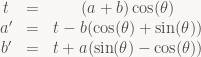
- Planar rotations. A bog-standard 2D rotation of the form
.
There’s not much to do about the butterflies, but the planar rotations are interesting, and different DCT algorithms use different ways of performing them. Let’s look at some:
Method 1: The obvious way
You can just do the matrix-vector multiply directly. Cost: 4 multiplies and 2 adds, or 2 multiplies and 2 FMAs.
Method 2: Saving a multiply
Rearranging the equation a bit allows us to extract a common factor:
For constant 
Note that there’s no special reason to base t off the cosine term, we could do the same with sin at the same cost:

Method 3: A scaled rotation
A different trick is used in the AA&N DCT (used by the IJG JPEG lib for the fast integer transform and the floating-point version):

Note that this is just Method 1 multiplied by 
(Again, there’s a dual version which multiplies by the cotangent of 
Method 4: Decompose into shears
There’s more: We can also write a rotation as three shears:

Note that this can be done without using any extra registers. Cost: 3 multiplies and 3 adds or 3 FMAs, but every operation is dependent on the previous one, so we get a chain of 3 dependent ops, same as for Method 2.
One interesting side effect of doing the computation this way is that the integer version of this is perfectly reversible, even if there are truncation errors in the multiplies – you just do the steps in reverse. Integer lifting formulations of wavelet transforms use the same primitive. One interesting consequence of this rotation formula is that it can be used to instantly obtain “integer lifting” versions of any orthogonal transform: You can compute the QR decomposition of any matrix using Givens rotations, which are just ordinary planar rotations and can be performed using this technique. If the matrix under consideration is orthogonal, then by uniqueness of the QR decomposition up to sign, we know that R is just a diagonal matrix with all entries being 1 or -1, so multiplication by R is perfectly reversible in integer values as well.
This nice property aside, the long dependency chains are somewhat bothersome. But it’s an interesting formula, and one that’s been used to design exactly reversible integer-to-integer DCTs (search for “BinDCT”).
Honorary mention: Complex multiply
There’s also a related formula to perform complex multiplication with just 3 multiplies instead of the usual 4 in the obvious formula

Compute it as

instead, using 3 multiplies and 5 adds. For a known fixed 
So which one do you use?
Well, I haven’t decided yet. For floating-point implementations on platforms with FMA support, method 3 is definitely the most attractive one, since absorbing scale factors into later butterflies is simple and doesn’t cause any trouble. Interestingly, both the very early Chen DCT factorization and the LL&M DCT factorization turn into algorithms with 22 FMAs and 4 adds when you apply this, and other FMA-optimized DCT algorithms use 26 ops as well. Interesting. Anyway, fixed-point is more bothersome: Every multiplication causes round-off error so you don’t want to have too many of them, or paths with a lot of multiplies in them. Also, multiplying by values with an absolute value larger than 1 (or 0.5, depending on the instruction set) is bothersome for fixed-point SIMD implementations. I haven’t decided yet what I’ll use.
Closing note: Don’t forget that arithmetic is only half of it – in this case, almost literally: I have a (untested, so beware) prototype implementation of a floating-point, FMA-based algorithm in a JPEG-like setting on Xbox 360. Half of the time in an 8×8 IDCT is actually spent doing the IDCT, the rest is loading, unpacking, tranposing, packing and storing. Still, the overall cost seems to be about 4.5 cycles per pixel (as said, not final code, so this might either increase or decrease by the time I’m done), so it’s not too bad. It also illustrates another point about image/video compression: The goddamn entropy coder ruins everything. 4.5 cycles per pixel for the IDCT is one thing, but you still have to decode the coefficients first. Chances are you need at least one variable-amount shift per coefficient during entropy decoding, and on the Cell/Xbox 360, these don’t come cheap – they’re microcoded, slow, and they block the second hardware thread while they run. And to add insult to injury, bitstream decoding is an inherently serial process while the rest is usable amenable to SIMD and parallelization. And yet none of our existing multimedia formats are designed to be efficiently decodeable using multiple cores; the current H.265 proposals started taking this into account, but virtually everything else is still completely serial. This particular bottleneck is going to stay with us for a long time.
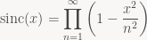
Another short one. This one bugged me for quite a while until I realized what the answer was a few years ago. The Sampling Theorem states that (under the right conditions)

where

(the normalized sinc function). The problem is this: Where does the sinc function come from? (In a philosophical sense. It plops out of the proof sure enough, but that’s not what I mean). Fourier theory is full of (trigonometric) polynomials (i.e. sine/cosine waves when you’re dealing with real-valued signals), so where does the factor of x in the denominator suddenly come from?
The answer is a nice identity discovered by Euler:
With some straightforward algebraic manipulations (ignoring convergence issues for now) you get:


Compare this with the formula for Lagrange basis polynomials:

in other words, the sinc function is the limiting case of Lagrange polynomials for an infinite number of equidistant control points. Which is pretty neat :)
Every time you ship a product with half-assed math in it, God kills a fluffy kitten by feeding it to an ill-tempered panda bear (don’t ask me why – I think it’s bizarre and oddly specific, but I have no say in the matter). There’s tons of ways to make your math way more complicated (and expensive) than it needs to be, but most of the time it’s the same few common mistakes repeated ad nauseam. Here’s a small checklist of things to look out for that will make your life easier and your code better:
- Symmetries. If your problem has some obvious symmetry, you can usually exploit it in the solution. If it has radial symmetry around some point, move that point to the origin. If there’s some coordinate system where the constraints (or the problem statement) get a lot simpler, try solving the problem in that coordinate system. This isn’t guaranteed to win you anything, but if you haven’t checked, you should – if symmetry leads to a solution, the solutions are usually very nice, clean and efficient.
- Geometry. If your problem is geometrical, draw a picture first, even if you know how to solve it algebraically. Approaches that use the geometry of the problem can often make use of symmetries that aren’t obvious when you write it in equations. More importantly, in geometric derivations, most of the quantities you compute actually have geometrical meaning (points, distances, ratios of lengths, etc). Very useful when debugging to get a quick sanity check. In contrast, intermediate values in the middle of algebraic manipulations rarely have any meaning within the context of the problem – you have to treat the solver essentially as a black box.
- Angles. Avoid them. They’re rarely what you actually want, they tend to introduce a lot of trigonometric functions into the code, you suddenly need to worry about parametrization artifacts (e.g. dealing with wraparound), and code using angles is generally harder to read/understand/debug than equivalent code using vectors (and slower, too).
- Absolute Angles. Particularly, never never ever use angles relative to some arbitrary absolute coordinate system. They will wrap around to negative at some point, and suddenly something breaks somewhere and nobody knows why. And if you’re about to introduce some arbitrary coordinate system just to determine some angles, stop and think very hard if that’s really a good idea. (If, upon reflection, you’re still undecided, this website has your answer).
- Did I mention angles? There’s one particular case of angle-mania that really pisses me off: Using inverse trigonometric functions immediately followed by sin / cos. atan2 / sin / cos: World’s most expensive 2D vector normalize. Using acos on the result of a dot product just to get the corresponding sin/tan? Time to brush up your trigonometric identities. A particularly bad offender can be found here – the relevant section from the simplified shader is this:
float alpha = max( acos( dot( v, n ) ), acos( dot( l, n ) ) );
float beta  = min( acos( dot( v, n ) ), acos( dot( l, n ) ) );
C = sin(alpha) * tan(beta);
Ouch! If you use some trig identities and the fact that acos is monotonically decreasing over its domain, this reduces to:
float vdotn = dot(v, n);
float ldotn = dot(l, n);
C = sqrt((1.0 - vdotn*vdotn) * (1.0 - ldotn*ldotn))
  / max(vdotn, ldotn);
..and suddenly there’s no need to use a lookup texture anymore (and by the way, this has way higher accuracy too). Come on, people! You don’t need to derive it by hand (although that’s not hard either), you don’t need to buy some formula collection, it’s all on Wikipedia – spend the two minutes and look it up!
- Elementary linear algebra. If you build some matrix by concatenating several transforms and it’s a performance bottleneck, don’t get all SIMD on it, do the obvious thing first: do the matrix multiply symbolically and generate the result directly instead of doing the matrix multiplies every time. (But state clearly in comments which transforms you multiplied together in what order to get your result or suffer the righteous wrath of the next person to touch that code). Don’t invert matrices that you know are orthogonal, just use the transpose! Don’t use 4×4 matrices everywhere when all your transforms (except for the projection matrix) are affine. It’s not rocket science.
- Unnecessary numerical differentiation. Numerical differentiation is numerically unstable, and notoriously difficult to get robust. It’s also often completely unnecessary. If you’re dealing with analytically defined functions, compute the derivative directly – no robustness issues, and it’s usually faster too (…but remember the chain rule if you warp your parameter on the way in).
Short version: Don’t just stick with the first implementation that works (usually barely). Once you have a solution, at least spend 5 minutes looking over it and check if you missed any obvious simplifications. If you won’t do it by yourself, think of the kittens!
More link-chasing! Charles has some more notes on the general “get center along axis” / “get radius along axis” primitives that are used in these tests. This is also at the heart of separating axis tests and the GJK algorithm for collision detection, so it’s definitely worth getting comfortable with. He also notes that:
Frustum culling is actually a bit subtle, in that how much work you should do on it depends on how expensive the object you are culling is to render. If the object will take 0.0001 ms to just render, you shouldn’t spend much time culling it. In that case you should use a simpler approximate test – for example a Cone vs. Sphere test. Or maybe no test at all – combine it into a group of objects and test the whole group of culling. If an object is very expensive to render (like maybe it’s a skinned human with very complex shaders), it takes 1 ms to render, then you want to cull it very accurately indeed – in fact you may want to test against an OBB or a convex hull of the object instead of just an AABB.
I agree with the second part, but I’m not sure about the cone vs. sphere test. Three reasons: First, the cone around the view frustum is really a pretty coarse approximation. For a 4:3 viewport, the area of the cone cross-section along the near plane is about 64% larger than the area of the bounding rectangle. For the 16:9 viewports we now commonly have it’s about 84% larger than the rect. That’s a very conservative test, even if you have tight-fitting bounding spheres. Second, even when an object is cheap to render, it still goes through a lot of pipeline stages before it ever gets submitted to the GPU. You don’t draw things immediately; you normally build a job list first that is then sorted. You may also do some sort of occlusion culling. For all survivors, you then need to set the state for that batch (shaders, constants, textures, various rendering states), do some state filtering while you’re at it (to avoid wasting GPU cycles with redundant state changes), and then finally issue the actual draw call. Even with optimized code, that’s usually a few thousand clock cycles start to finish. For posterity, let’s assume that the box-frustum test costs 50 cycles more than a sphere-cone test (which is generous), and each non-culled batch costs an average of 1000 cycles start to finish. If your coarse test has a false positive rate of only 5%, it’s no win; at 10%, it’s a 50 cycles/batch net cost. Third, even if it is a win on the CPU side, you end up generating GPU work for some false positives. Wasted GPU cycles are more expensive than wasted CPU cycles, because there’s less of them (lower clock rate, and usually just one GPU vs. more than one CPU core nowadays).
Grouping is a good point though. If there’s a natural grouping for your dynamic objects, exploit it. For your scenery, you should build a static hierarchy. Large cache lines, high mispredicted branch penalties and SIMD-optimized processors mean that any kind of binary tree is a bad choice (doubly so when you don’t have fast random access to memory as on SPUs). Use a larger fan-out, aim for a fairly flat hierarchy (again, doubly so for SPUs). Don’t build just any tree; use a simple cost function and choose your subdivisions to minimize it (no need for exhaustive search, it’s enough to test 5-8 different options at each level and pick the best one). If in doubt, build a binary hierarchy first (it’s easier to code) then merge nodes later to get the larger fan-out.
Culling tests inside a hierarchy have different trade-offs than the per-batch culling tests you do at the leaf nodes, so consider using different code (or a different type of bounding volume) for it.
If your tests work with clipspace geometry, it’s fairly easy to build a 2D screen-space bounding box around your BV while you’re at it. The cheap version just returns the whole screen when the BV crosses the near plane; Blinn describes a more accurate (but slower) variant in “Calculating Screen Coverage” (Chapter 6 of “Jim Blinn’s Corner: Notation, Notation, Notation”, another book you should consider buying). Either way, this bbox is useful: you can use it to estimate the screen size of objects (useful for LOD selection and to reject objects entirely once they’re smaller than a few pixels) and as input to a coarse occlusion test.
The bbox screen size test is more generally useful than a far-plane test; if you use it, consider skipping the far-plane test entirely during your per-batch culling. That brings your plane count down to 5; depending on your geometry, there might be another plane that’s not really helpful for culling (usually the top or bottom plane). Throwing another plane out gets you down to 4, which may or may not make your culling code nicer (4-way SIMD and all). Debatable whether it helps nowadays, but it used to be nifty on PS2 :)
Recently stumbled across this series by Zeux. It’s well written, but I have one tiny objection about the content. The money quote is in part 5, where he says that “there is p/n-vertex approach which I did not implement (but I’m certain that it won’t be a win over my current methods on SPUs)”. Hoo boy. Being certain about something you don’t know is never a good strategy in programming (or life in general for that matter). View-frustum culling for AABBs is something I’ve come across multiple times in the 12 years that I’ve been seriously doing 3D graphics. There’s tons of nice tricks of the trade, and even though all of them are published somewhere, most people don’t bother looking it up (after all, the obvious algorithm is simple enough and not very slow) – incidentally, there’s two books that are most likely already in your office somewhere (if you’re a graphics or game programmer) that you should consult on the topic: “Real-Time Rendering” (16.10, “Plane/Box Intersection Detection”) and “Real-Time Collision Detection” (5.2.3, “Testing Box Against Plane”). Both describe a very slick implementation of the “p/n-vertex” approach. But I’m gonna take a trip down memory lane and explain the various approaches I’ve been using over the years (don’t expect optimized implementations of all of them, I’m just going to explain the basic idea of each test and then move on, for the most part).
Read more…
Two discoveries from recent months. The first one was on x86-64 and occurs in this code fragment:
U32 offset = ...;
U8 *ptr = base + (offset & 0xffff)*4;
I expected to get one “and”, with the rest folded into an address computation (after all, x86 has a base+index*4 addressing mode). What I actually got was this:
; eax = offset, rcx=base
movzx eax, ax ; equivalent to "and eax, 0ffffh" (but smaller)
shl   eax, 2
add   rax, rcx
The operand size mismatch between the instructions is the clue – the compiler computes the “*4” in 32 bits; the “*4” in an address computation would be computed for 64-bit temporaries. This is a result of the C/C++ typing rules: All of (offset & 0xffff) * 4 is computed as “unsigned int”, since C does most computations at “int” size, which is 32 bits even on most 64-bit platforms. The compiler can’t use the built-in “*4” addressing mode since (U32) x*4 isn’t equivalent to (U64) x*4 in the presence of overflow (of course, in the example given, we can’t ever get any overflows, but that’s something that the optimizer apparently wasn’t looking for).
Easy solution: use U8 *ptr = base + U64(offset & 0xffff)*4 (alternatively, multiply by “4ull” or “(size_t) 4”) and everything comes out as expected. But it illustrates an interesting dilemma: In the simpler expression U8 *ptr = base + offset*4, would you have expect the “offset*4” part to be computed in 32 bits? Probably not. “int” was left at 32-bits since a lot of code relies on it, and most ints we use really don’t need more than 32 bits. But the type conversion rules in C/C++ implicitly assume that an “int” is the native register type, leading to this kind of problem when that’s not the case. Right now, virtually nobody uses single arrays larger than 4GB, but it’s only a matter of time until that changes…
Anyway, on to tidbit number two, which concerns GCC on PS3 (PPU code). The PPU is a 64-bit PowerPC processor, but the PS3 has only 256MB of RAM (plus 256MB of graphics memory), so there’s no reason to use 64-bit pointers – it’s just a waste of memory. And again, overflow makes everything complicated. GCC assumes that (almost) all address computations could overflow at any time. It thus tends to perform address calculations manually and clear the top 32 bits afterwards, instead of using the built-in addressing modes of the CPU. This produces code that’s significantly larger (and slower) than necessary. To give an example, take this piece of code:
U32 *p = ...;
*++p = x;
*++p = y;
A good translation of this code into PPC assembly looks like this: (with explanation in case you don’t know PPC assembly)
; r8=p, r9=x, r10=y
stw  r9, 4(r8)   ; *(p + 1) = x;
stwu r10, 8(r8)  ; *(p + 2) = y; p += 2;
but what GCC actually produces for this code sequence looks more like this:
addi   r11, r8, 4   ; t = p + 1;
addi   r8, r8, 8    ; p += 2;
clrldi r11, r11, 32 ; clear top 32 bits of t
clrldi r8, r8, 32   ; same for p
stw    r9, 0(r11)   ; *t = x;
stw    r10, 0(r8)   ; *p = y;
Note that it’s not only 3x the number of instructions, but also needs extra registers (thus increasing register pressure). It’s the same underlying problem as with the x86 example – a lot of extra work to enforce artificial wraparound of 32-bit quantities. A pretty dubious goal, since it’s very unlikely that code actually wants that 32-bit wraparound (and if it does, it should probably be fixed), but I digress… Anyway, it turns out that there’s one case where GCC assumes that pointers won’t wrap around: Structure accesses. So in this case:
struct Blah {
  U32 x, y;
};

Blah *p = ...;
p->x = x;
p->y = y;
You’ll actually get reasonable code without an addi/clrldi combo for every access. So if you’re writing out a stream of words (something that’s fairly common when building a rendering command buffer), you can save a lot of instructions by declaring a simple struct:
struct CommandData {
  U32 w0, w1, w2, w3, w4, w5, w6, w7;
};
and then replacing this kind of code:
U32 *cmd = ...;
cmd[0] = foo;
cmd[1] = bar;
cmd[2] = blah;
cmd[3] = blub;
cmd += 4;
with the (admittedly somewhat obscure-looking)
CommandData *cmd_out = (CommandData *) cmd;
cmd_out->w0 = foo;
cmd_out->w1 = bar;
cmd_out->w2 = blah;
cmd_out->w3 = blub;
cmd = &cmd_out->w4;
This is only useful to know if you’re programming on PS3 and using GCC, but if you do, that kind of stuff can make a big difference. I’ve recently been working a lot on PS3 rendering code and got speedups in excess of 10% from this and other low-level optimizations along the same vein. Actually reading the assembly generated by your compiler is important, especially when targeting in-order CPUs. It’s nearly impossible to see this kind of problem when you’re thinking at the level of C/C++ source code.
What the title says :). Just thought it was worth mentioning since I talked a bit about singly-linked lists in the “Data structures and invariants” post, and cycles are the primary way that a singly-linked list can “go wrong” on you without containing invalid pointers: notably, you can get this if you try to insert some item x to a list when that list already contains x. (If you insert the “new” x before or at the position of the x that’s already in the list, you will get a cycle. If you insert it later, you will inadvertently remove all items between the old and new position).
When debugging this, it’s useful to have some cycle-detection code. You can add some fields to the list for debugging (not quite as trivial as it sounds, since clearing a “visited” flag involves traversing the list that might have a cycle – you need to make sure all fields are in a known “visited” state before you start looking for cycles if you do it this way), but a nicer solution that doesn’t require extra memory is to use a cycle detection algorithm. There are two main choices – Floyd’s “tortoise and hare” algorithm and Brent’s algorithm – and both are worth knowing about. They’re also explained well on Wikipedia, so read up if you’ve never encountered them before.
Following Google’s announcement of WebP, there’s been a lot of (justified) criticism of it based on its merits as an image coder. As a compression geek, I’m interested, but as both a creator and consumer of digital media formats, my main criticism is something else entirely: The last thing we need is yet another image format. This was already true when JPEG 2000 and JPEG XR were released. Never mind that their purported big compression advantages were greatly exaggerated (and based on dubious metrics); even if the standards had delivered clear-cut improvements on that front, they would’ve been irrelevant. Improved compression rate is not a feature. Not by itself, anyway. As someone who deals with content, I care about compression rate only as long as size is a limiting factor. As someone taking photos, I care whether all the pictures I shoot in one day fit onto my camera. Back when digital cameras were crappy, had low resolution and a tiny amount of storage, the JPEG compression made a big difference. Nowadays, we have 8 Megapixel cameras and multiple Gigabytes of storage in our cellphones. For normal usage, I can shoot RAW photos all day long and still not exhaust the space available to me. It’s done, problem solved. I might care about the size reduction once I start archiving stuff, but again, the 10:1 I get with plain JPEG at decent quality is plenty – a guaranteed 30% improvement on top of that (which JPEG2k/JPEG-XR/WebP don’t deliver!) is firmly into “don’t care” territory. It doesn’t solve any real problem.
The story is the same way for audio. MP3 offered an reduction of about 10:1 for CD quality audio at the right time, and made digitally archiving music practical. And we still gladly take the 10:1 on everything, since fitting 10x more on our MP3 players is convenient. But again, that’s only a factor of storage limitations that are rapidly disappearing. MP3 players started getting popular because they were smaller than mobile CD players and could (gosh!) store multiple albums worth of music (of course, back then “multiple albums” was a number in the single digits, and only if you compressed them greatly). Nowadays, most people can easily fit their complete music collection onto an iPod (or, again, their cellphone). Give it another 5 years and you’ll have enough space to fit it in as uncompressed WAV files if you choose to (not going to happen since most people now get music directly in MP3/AAC format, but it would be possible). Again, problem solved. Better audio compression remains an interesting problem with lots of fascinating ties to perception and psychology, but there’s just no real practical need for better audio compression these days. Audio just isn’t that much data.
Video is about the only mainstream type of content where the compression ratio still matters: 1080i60 video (as used in sports broadcasts for example) is about 90 megabytes per second in the subsamples YUV 4:2:0 color space it typically comes in, and about 350MB/s in the de-interlaced RGB color space we use for display. That’s unwieldy enough to need some serious compression (and partial or complete hardware support for decompression). And even the compressed representations are large enough to be unwieldy (we stick them onto Blu-ray discs and worry about the video streaming costs). So there’s still some future for innovation there, but even that window is rapidly closing. Blu-ray is probably the last disc format that was motivated partly by the need to store the amount of content needed for high-fidelity video. HDTV resolutions are gonna stay with us for a good while (HD is close enough to the internal resolutions used in movie production to make any further improvements subject to rapidly diminishing returns), and Blu-rays are already large enough to store HD content with good quality using current codec technology. BDXL is on the way; again, that’s just large enough for what we want to do with it. The next generation of video codecs after H.264 is probably still going to matter, since video is still a shitload of data right now. But we’ve been getting immensely better at large-scale image and signal processing (mainly with sheer brute force) and Moore’s law works in our favor. Five years ago, digital video was something done mainly by professionals and enthusiasts with the willingness to invest into expensive hardware. Nowadays, you can get cheap HD camcorders and do video postproduction on a normal laptop, if you’re willing to stomach the somewhat awkward workflow and long processing times. Ten years from now, a single 720p video will be something you can deal with as a matter of course on any device, just as you do with a single MP3 nowadays (…remember when encoding them took 2x as long as their runtime? Yeah, that was just 10 years ago).
And in the meantime, the last thing we need is yet more mutually incompatible formats with different feature sets and representations to make the lives of everyone dealing with this crap a living hell. If you don’t have any actual, useful features to offer (a standard lossy format with alpha channel would be nice, as would HDR support in a mainstream format) just shut up already.
Enough bit-twiddling for now, time to talk about something a bit more substantial: Invariants. If you don’t know what that is, an invariant is just a set of conditions that will hold before and after every “step” of your program/algorithm. This is usually taught in formal CS education, but textbooks love to focus on invariants in algorithm design. That’s fine for the types of algorithms typically found (and analyzed) en masse in CS textbooks: sorting, searching, and basic graph algorithms. But it has little relevance to the type of problems you usually encounter in applications, where you don’t encounter nice abstract problems with well-defined input and output specifications, but a tangled mess of several (often partially conflicting) requirements that you have to make sense of. So most programmers forget about invariants pretty soon and don’t think about them again.
That’s a mistake. Invariants are a very useful tool in practice, if you have a clear specification of what’s supposed to happen, and how. That may not be the case for the whole of the program, but it’s usually the case for the part of your code that manipulates data structures. Let me give you some examples: Read more…
