rANS notes

We’ve been spending some time at RAD looking at Jarek Duda’s ANS/ABS coders (paper). This is essentially a new way of doing arithmetic coding with some different trade-offs from the standard methods. In particular, they have a few sweet spots for situations that were (previously) hard to handle efficiently with regular arithmetic coding.

The paper covers numerous algorithms. Of those given, I think what Jarek calls “rANS” and “tANS” are the most interesting ones; there’s plenty of binary arithmetic coders already and “uABS”, “rABS” or “tABS” do not, at first sight, offer any compelling reasons to switch (that said, there’s some non-obvious advantages that I’ll get to in a later post).

Charles has already posted a good introduction; I recommend you start there. Charles has also spent a lot of time dealing with the table-based coders, and the table-based construction allows some extra degrees of freedom that make it hard to see what’s actually going on. In this post, I’m going to mostly talk about rANS, the range coder equivalent. Charles already describes it up to the point where you try to make it “streaming” (i.e. finite precision); I’m going to continue from there.

Streaming rANS

In Charles’ notation (which I’m going to use because the paper uses both indexed upper-case I’s and indexed lower-case l’s, which would make reading this with the default font a disaster), we have two functions now: The coding function C and the decoding function D defined as

where .

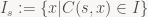
D determines the encoded symbol s by looking at (x mod M) and looking up the corresponding value in our cumulative frequency table (s is the unique s such that ).

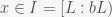
Okay. If you're working with infinite-precision integers, that's all you need, but that's not exactly suitable for fast (de)compression. We want a way to perform this using finite-precision integers, which means we want to limit the size of x somehow. So what we do is define a "normalized" interval

The [L:bL) thing on the right is the notation I'll be using for a half-open interval of integers). b is the radix of our encoder; b=2 means we're emitting bits at a time, b=256 means we're emitting bytes, and so forth. Okay. We now want to keep x in this range. Too large x don't fit in finite-precision integers, but why not allow small x? The (hand-wavey) intuition is that too small x don't contain enough information; as Charles mentioned, x essentially contains about bits of information. If x < 4, it can only be one of four distinct values, and as you saw above the value of x (mod M) directly determines which symbol we're coding. So we want x just right: not too large, not too small. Okay. Now let's look at how a corresponding decoder would look:

  while (!done) {
    // Loop invariant: x is normalized.
    assert(L <= x && x < b*L);

    // Decode a symbol
    s, x = D(x);

    // Renormalization: While x is too small,
    // keep reading more bits (nibbles, bytes, ...)
    while (x < L)
      x = x*b + readFromStream();
  }

Turns out that’s actually our decoding algorithm, period. What we need to do now is figure out how the corresponding encoder looks. As long as we’re only using C and D with big integers, it’s simple; the two are just inverses of each other. Likewise, we want our encoder to be the inverse of our decoder – exactly. That means we have to do the inverse of the operations the decoder does, in the opposite order. Which means our encoder has to look something like this:

  while (!done) {
    // Inverse renormalization: emit bits/bytes etc.
    while (???) {
      writeToStream(x % b);
      x /= b;
    }

    // Encode a symbol
    x = C(s, x);
 
    // Loop invariant: x is normalized
    assert(L <= x && x < b*L);
  }

So far, this is purely mechanical. The only question is what happens in the “???” – when exactly do we emit bits? Well, for the encoder and decoder to be inverses of each other, the answer has to be “exactly when the decoder would read them”. Well, the decoder reads bits whenever the normalization variant is violated after decoding a symbol, to make sure it holds for the next iteration of the loop. The encoder, again, needs to do the opposite – we need to proactively emit bits before coding s to make sure that, after we’ve applied C, x will be normalized.

In fact, that’s all we need for a first sketch of renormalization:

  while (!done) {
    // Keep trying until we succeed
    for (;;) {
      x_try = C(s, x);
      if (L <= x_try && x_try < b*L) { // ok?
        x = x_try;
        break;
      } else {
        // Shrink x a bit and try again
        writeToStream(x % b);
        x /= b;
      }
    }

    x = x_try;
  }

Does this work? Well, it might. It depends. We certainly can’t guarantee it from where we’re standing, though. And even if it does, it’s kind of ugly. Can’t we do better? What about the normalization – I’ve just written down the normalization loops, but just because both decoder and encoder maintain the same invariants doesn’t necessarily mean they are in sync. What if at some point of the loop, there are more than two possible normalized configurations – can this happen? Plus there’s some hidden assumptions in here: the encoder, by only ever shrinking x before C, assumes that C always causes x to increase (or at least never causes x to decrease); similarly, the decoder assumes that applying D won’t increase x.

And I’m afraid this is where the proofs begin.

Streaming rANS: the proofs (part 1)

Let’s start with the last question first: does C always increase x? It certainly looks like it might, but there’s floors involved – what if there’s some corner case lurking? Time to check:

since , , and are all non-negative (the latter because – each symbol's frequency is less than the sum of all symbol frequencies). So C indeed always increases x, or more precisely, never decreases it.

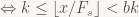
Next up: normalization. Let's tackle the decoder first. First off, is normalization in the decoder unique? That is, if , is that the only normalized x it could be at that stage in the decoding process? Yes, it is: , so , so

where arbitrary

That is, no matter what bit / byte / whatever the decoder would read next (that's 'd'), running through the normalization loop once more would cause x to become too large; there's only one way for x to be normalized. But do we always end up with a normalized x? Again, yes. Suppose that , then (because we're working in integers) , and hence

(again arbitrary)

The same kind of argument works for the encoder, which floor-divides by b instead of multiplying b it. The key here is that our normalization interval I has a property the ANS paper calls “b-uniqueness”: it’s of the form for some positive integer k (its upper bound is b times its lower bound). Any process that grows (or shrinks) x in multiples of b can’t “skip over” I (as in, transition from being larger than the largest value in I to smaller than the smallest value in I or vice versa) in a single step. Simultaneously, there’s also never two valid states the encoder/decoder could be in (which could make them go out of sync: both encoder and decoder think they’re normalized, but they’re at different state values).

To elaborate, suppose we have b=2 and some interval where the ratio between lower and upper bound is a tiny bit less than 2: say There’s just one value missing. Now suppose the decoder is in state and reads a bit, which turns out to be 1. Then the new state is – we overshot! We were below the lower bound of I’, and yet with a single bit read, we’re now past its upper bound. I’ is “too small”.

Now let’s try the other direction; again b=2, and this time we make the ratio between upper and lower bound a bit too high: set There’s no risk of not reaching a state in that interval now, but now there is ambiguity. Where’s the problem? Suppose the encoder is in state . Coding any symbol will require renormalization to “shift out” one bit. The encoder writes that bit (a zero), goes to state , and moves on. But there’s a problem: the decoder, after decoding that symbol, will be in state too. And it doesn’t know that the encoder got there from state by shifting a bit; all the decoder knows is that it’s in state , which is normalized and doesn’t require reading any more bits. So the encoder has written a bit that the decoder doesn’t read, and now the two go out of sync.

Long story short: if the state intervals involved aren’t b-unique, bad things happen. And on the subject of bad things happening, our encoder tries to find an x such that C(s,x) is inside I by shrinking x – but what if that process doesn't find a suitable x? We need to know a bit more about which values of x lead to C(s,x) being inside I, which leads us to the sets

i.e. the set of all x such that encoding 's' puts us into I again. If all these sets turn out to be b-unique intervals, we're good. If not, we're in trouble. Time for a brief example.

Intermission: why b-uniqueness is necessary

Let’s pick L=5, b=2 and M=3. We have just two symbols: ‘a’ has probability , and ‘b’ has probability , which we turn into , , , . Our normalization interval is . By computing C(s,x) for the relevant values of s and x, we find out that

Uh-oh. Neither of these two intervals is b-unique. is too small, and is too big. So what goes wrong?

Well, suppose that we’re in state x=7 and want to encode an ‘a’. 7 is not in (too large). So the encoder emits the LSB of x, divides by 2 and… now x=3. Well, that’s not in either (too small), and shrinking it even further won’t help that. So at this point, the encoder is stuck; there’s no x it can reach that works.

Proofs (part 2): a sufficient condition for b-uniqueness

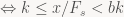
So we just saw that in certain scenarios, rANS can just get stuck. Is there anything we can do to avoid it? Yes: the paper points out that the embarrassing situation we just ran into can’t happen when M (the sum of all symbol frequencies, the denominator in our probability distribution) divides L, our normalization interval lower bound. That is, for some positive integer k. It doesn’t give details, though; so, knowing this, can we prove anything about the that would help us? Well, let’s just look at the elements of and see what we can do:

let’s work on that condition:

at this point, we can use that and divide by M:

Now, for arbitrary real numbers r and natural numbers n we have that

Using this, we get:

note the term in the outer floor bracket is the sum of an integer and a real value inside , since , so we can simplify drastically

where we applied the floor identities above again and then just multiplied by . Note that the result is an interval of integers with its (exclusive) upper bound being equal to b times its (inclusive) lower bound, just like we need – in other words, assuming that , all the are b-unique and we're golden (this is mentioned in the paper in section 3.3, but not proven, at least not in the Jan 6 2014 version).

Note that this also gives us a much nicer expression to check for our encoder. In fact, we only need the upper bound (due to b-uniqueness, we know there's no risk of us falling through the lower bound), and we end up with the encoding function

  while (!done) {
    // Loop invariant: x is normalized
    assert(L <= x && x < b*L);

    // Renormalize
    x_max = (b * (L / M)) * freq[s]; // all but freq[s] constant
    while (x >= x_max) {
      writeToStream(x % b);
      x /= b;
    }

    // Encode a symbol
    // x = C(s, x);
    x = freq[s] * (x / M) + (x % M) + base[s];
  }

No “???”s left – we have a “streaming” (finite-precision) version of rANS, which is almost like the arithmetic coders you know and love (and in fact quite closely related) except for the bit where you need to encode your data in reverse (and reverse the resulting byte stream).

I put an actual implementation on Github for the curious.

Some conclusions

This is an arithmetic coder, just a weird one. The reverse encoding seems like a total pain at first, and it kind of is, but it comes with a bunch of really non-obvious but amazing advantages that I’ll cover in a later post (or just read the comments in the code). The fact that M (the sum of all frequencies) has to be a multiple of L is a serious limitation, but I don’t (yet?) see any way to work around that while preserving b-uniqueness. So the compromise is to pick M and L to be both powers of 2. This makes the decoder’s division/mod with M fast. The power-of-2 limitation makes rANS really bad for adaptive coding (where you’re constantly updating your stats, and resampling to a power-of-2-sized distribution is expensive), but hey, so is Huffman. As a Huffman replacement, it’s really quite good.

In particular, it supports a divide-free decoder (and actually no per-symbol division in the encoder either, if you have a static table; see my code on Github, RansEncPutSymbol in particular). This is something you can’t (easily) do with existing multi-symbol arithmetic coders, and is a really cool property to have, because it really puts it a lot closer to being a viable Huffman replacement in a lot of places that do care about the speed.

If you look at the decoder, you’ll notice that its entire behavior for a decoding step only depends on the value of x at the beginning: figure out the symbol from the low-order bits of x, go to a new state, read some bits until we’re normalized again. This is where the table-based versions (tANS etc.) come into play: you can just tabulate their behavior! To make this work, you want to keep b and L relatively small. Then you just make a table of what happens in every possible state.

Interestingly, because these tables really do tabulate the behavior of a “proper” arithmetic coder, they’re compatible: if you have two table-baked distributions with use that same values of b and L (i.e. the same interval I), you can switch between them freely; the states mean the same in both of them. It’s not at all obvious that it’s even possible for a table-based encoder to have this property, so it’s even cooler that it comes with no onerous requirements on the distribution!

That said, as interesting as the table-based schemes are, I think the non-table-based variant (rANS) is actually more widely useful. Having small tables severely limits your probability resolution (and range precision), and big tables are somewhat dubious: adds, integer multiplies and bit operations are fine. We can do these quickly. More compute power is a safe thing to bet on right now (memory access is not). (I do have some data points on what you can do on current HW, but I’ll get there in a later post.)

As said, rANS has a bunch of really cool, unusual properties, some of which I’d never have expected to see in any practical entropy coder, with cool consequences. I’ll put that in a separate post, though – this one is long (and technical) enough already. Until then!