The care and feeding of worker threads, part 1

This post is part of a series – go here for the index.

It’s time for another post! After all the time I’ve spent on squeezing about 20% out of the depth rasterizer, I figured it was time to change gears and look at something different again. But before we get started on that new topic, there’s one more set of changes that I want to talk about.

The occlusion test rasterizer

So far, we’ve mostly been looking at one rasterizer only – the one that actually renders the depth buffer we cull against, and even more precisely, only multi-threaded SSE version of it. But the occlusion culling demo has two sets of rasterizers: the other set is used for the occlusion tests. It renders bounding boxes for the various models to be tested and checks whether they are fully occluded. Check out the code if you’re interested in the details.

This is basically the same rasterizer that we already talked about. In the previous two posts, I talked about optimizing the depth buffer rasterizer, but most of the same changes apply to the test rasterizer too. It didn’t make sense to talk through the same thing again, so I took the liberty of just making the same changes (with some minor tweaks) to the test rasterizer “off-screen”. So, just a heads-up: the test rasterizer has changed while you weren’t looking – unless you closely watch the Github repository, that is.

And now that we’ve established that there’s another inner loop we ought to be aware of, let’s zoom out a bit and look at the bigger picture.

Some open questions

There’s two questions you might have if you’ve been following this series closely so far. The first concerns a very visible difference between the depth and test rasterizers that you might have noticed if you ran the code. It’s also visible in the data in “Depth buffers done quick, part 1”, though I didn’t talk about it at the time. I’m talking, of course, about the large standard deviation we get for the execution time of the occlusion tests. Here’s a set of measurements for the code right after bringing the test rasterizer up to date:

Pass	min	25th	med	75th	max	mean	sdev
Render depth	2.666	2.716	2.732	2.745	2.811	2.731	0.022
Occlusion test	1.335	1.545	1.587	1.631	1.761	1.585	0.066

Now, the standard deviation actually got a fair bit lower with the rasterizer changes (originally, we were well above 0.1ms), but it’s still surprisingly large, especially considering that the occlusion tests run roughly half as long (in terms of wall-clock time) as the depth rendering. And there’s also a second elephant in the room that’s been staring us in the face for quite a while. Let me recycle one of the VTune screenshots from last time:

Right there at #4 is some code from TBB, namely, what turns out to be the “thread is idle” spin loop.

Well, so far, we’ve been profiling, measuring and optimizing this as if it was a single-threaded application, but it’s not. The code uses TBB to dispatch tasks to worker threads, and clearly, a lot of these worker threads seem to be idle a lot of the time. But why? To answer that question, we need a bit different information than what either a normal VTune analysis run or our summary timers give us. We want a detailed breakdown of what happens during a frame. Now, VTune has some support for that (as part of their threading/concurrency profiling), but the UI doesn’t work well for me, and neither does the the visualization; it seems to be geared towards HPC/throughput computing more than latency-sensitive applications like real-time graphics, and it’s also still based on sampling profiling, which means it’s low-overhead but fairly limited in the kind of data it can collect.

Instead, I’m going to go for the shameless plug and use Telemetry instead (full disclosure: I work at RAD). It works like this: I manually instrument the source code to tell Telemetry when certain events are happening, and Telemetry collects that data, sends the whole log to a server and can later visualize it. Most games I’ve worked on have some kind of “bar graph profiler” that can visualize within-frame events, but because Telemetry keeps the whole data stream, it can also be used to answer the favorite question (not!) of engine programmers everywhere: “Wait, what the hell just happened there?”. Instead of trying to explain it in words, I’m just gonna show you the screenshot of my initial profiling run after I hooked up Telemetry and added some basic markup: (Click on the image to get the full-sized version)

The time axis goes from left to right, and all of the blocks correspond to regions of code that I’ve marked up. Regions can nest, and when they do, the blocks stack. I’m only using really basic markup right now, because that turns out to be all we need for the time being. The different tracks correspond to different threads.

As you can see, despite the code using TBB and worker threads, it’s fairly rare for more than 2 threads to be actually running anything interesting at a time. Also, if you look at the “Rasterize” and “DepthTest” tasks, you’ll notice that we’re spending a fair amount of time just waiting for the last 2 threads to finish their respective jobs, while the other worker threads are idle. That’s where our variance in latency ultimately comes from – it all depends on how lucky (or unlucky) we get with scheduling, and the exact scheduling of tasks changes every frame. And now that we’ve seen how much time the worker threads spend being idle, it also shouldn’t surprise us that TBB’s idle spin loop ranked as high as it did in the profile.

What do we do about it, though?

Let’s start with something simple

As usual, we go for the low-hanging fruit first, and if you look at the left side of the screenshot I’ll posted, you’ll see a lot of blocks (“zones”) on the left side of the screen. In fact, the count is much higher than you probably think – these are LOD zones, which means that Telemetry has grouped a bunch of very short zones into larger groups for the purposes of visualization. As you can see from the mouse-over text, the single block I’m pointing at with the mouse cursor corresponds to 583 zones – and each of those zones corresponds to an individual TBB task! That’s because this culling code uses one TBB task per model to be culled. Ouch. Let’s zoom in a bit:

Note that even at this zoom level (the whole screen covers about 1.3ms), most zones are still LOD’d out. I’ve mouse-over’ed on a single task that happens to hit one or two L3 cache miss and so is long enough (at about 1500 cycles) to show up individually, but most of these tasks are closer to 600 cycles. In total, frustum culling the approximately 1600 occluder models takes up just above 1ms, as the captions helpfully say. For reference, the much smaller block that says “OccludeesVisible” and takes about 0.1ms? That one actually processes about 27000 models (it’s the code we optimized in “Frustum culling: turning the crank”). Again, ouch.

Fortunately, there’s a simple solution: don’t use one task per model. Instead, use a smaller number of tasks (I just used 32) that each cover multiple models. The code is fairly obvious, so I won’t bother repeating it here, but I am going to show you the results:

Down from 1ms to 0.08ms in two minutes of work. Now we could apply the same level of optimization as we did to the occludee culling, but I’m not going to bother, because at least not for the time being it’s fast enough. And with that out of the way, let’s look at the rasterization and depth testing part.

A closer look

Let’s look a bit more closely at what’s going on during rasterization:

There are at least two noteworthy things clearly visible in this screenshot:

1. There’s three separate passes – transform, bin, then rasterize.
2. For some reason, we seem to have an odd mixture of really long tasks and very short ones.

The former shouldn’t come as a surprise, since it’s explicit in the code:

gTaskMgr.CreateTaskSet(&DepthBufferRasterizerSSEMT::TransformMeshes, this,
    NUM_XFORMVERTS_TASKS, NULL, 0, "Xform Vertices", &mXformMesh);
gTaskMgr.CreateTaskSet(&DepthBufferRasterizerSSEMT::BinTransformedMeshes, this,
    NUM_XFORMVERTS_TASKS, &mXformMesh, 1, "Bin Meshes", &mBinMesh);
gTaskMgr.CreateTaskSet(&DepthBufferRasterizerSSEMT::RasterizeBinnedTrianglesToDepthBuffer, this,
    NUM_TILES, &mBinMesh, 1, "Raster Tris to DB", &mRasterize);	

// Wait for the task set
gTaskMgr.WaitForSet(mRasterize);

What the screenshot does show us, however, is the cost of those synchronization points. There sure is a lot of “air” in that diagram, and we could get some significant gains from squeezing it out. The second point is more of a surprise though, because the code does in fact try pretty hard to make sure the tasks are evenly sized. There’s a problem, though:

void TransformedModelSSE::TransformMeshes(...)
{
    if(mVisible)
    {
        // compute mTooSmall

        if(!mTooSmall)
        {
            // transform verts
        }
    }
}

void TransformedModelSSE::BinTransformedTrianglesMT(...)
{
    if(mVisible && !mTooSmall)
    {
        // bin triangles
    }
}

Just because we make sure each task handles an equal number of vertices (as happens for the “TransformMeshes” tasks) or an equal number of triangles (“BinTransformedTriangles”) doesn’t mean they are similarly-sized, because the work subdivision ignores culling. Evidently, the tasks end up not being uniformly sized – not even close. Looks like we need to do some load balancing.

Balancing act

To simplify things, I moved the computation of mTooSmall from TransformMeshes into IsVisible – right after the frustum culling itself. That required some shuffling arguments around, but it’s exactly the kind of thing we already saw in “Frustum culling: turning the crank”, so there’s little point in going over it in detail again.

Once TransformMeshes and BinTransformedTrianglesMT use the exact same condition – mVisible && !mTooSmall – we can determine the list of models that are visible and not too small once, compute how many triangles and vertices these models have in total, and then use these corrected numbers which account for the culling when we’re setting up the individual transform and binning tasks.

This is easy to do: DepthBufferRasterizerSSE gets a few more member variables

UINT *mpModelIndexA; // 'active' models = visible and not too small
UINT mNumModelsA;
UINT mNumVerticesA;
UINT mNumTrianglesA;

and two new member functions

inline void ResetActive()
{
    mNumModelsA = mNumVerticesA = mNumTrianglesA = 0;
}

inline void Activate(UINT modelId)
{
    UINT activeId = mNumModelsA++;
    assert(activeId < mNumModels1);

    mpModelIndexA[activeId] = modelId;
    mNumVerticesA += mpStartV1[modelId + 1] - mpStartV1[modelId];
    mNumTrianglesA += mpStartT1[modelId + 1] - mpStartT1[modelId];
}

that handle the accounting. The depth buffer rasterizer already kept cumulative vertex and triangle counts for all models; I added one more element at the end so I could use the simplified vertex/triangle-counting logic.

Then, at the end of the IsVisible pass (after the worker threads are done), I run

// Determine which models are active
ResetActive();
for (UINT i=0; i < mNumModels1; i++)
    if(mpTransformedModels1[i].IsRasterized2DB())
        Activate(i);

where IsRasterized2DB() is just a predicate that returns mIsVisible && !mTooSmall (it was already there, so I used it).

After that, all that remains is distributing work over the active models only, using mNumVerticesA and mNumTrianglesA. This is as simple as turning the original loop in TransformMeshes

for(UINT ss = 0; ss < mNumModels1; ss++)

into

for(UINT active = 0; active < mNumModelsA; active++)
{
    UINT ss = mpModelIndexA[active];
    // ...
}

and the same for BinTransformedMeshes. All in all, this took me about 10 minutes to write, debug and test. And with that, we should have proper load balancing for the first two passes of rendering: transform and binning. The question, as always, is: does it help?

Change: Better rendering “front end” load balancing

Version	min	25th	med	75th	max	mean	sdev
Initial depth render	2.666	2.716	2.732	2.745	2.811	2.731	0.022
Balance front end	2.282	2.323	2.339	2.362	2.476	2.347	0.034

Oh boy, does it ever. That’s a 14.4% reduction on top of what we already got last time. And Telemetry tells us we’re now doing a much better job at submitting uniform-sized tasks:

In this frame, there’s still one transform batch that takes longer than the others; this happens sometimes, because of context switches for example. But note that the other threads nicely pick up the slack, and we’re still fine: a ~2x variation on the occasional item isn’t a big deal, provided most items are still roughly the same size. Also note that, even though there’s 8 worker threads, we never seem to be running more than 4 tasks at a time, and the hand-offs between threads (look at what happens in the BinMeshes phase) seem too perfectly synchronized to just happen accidentally. I’m assuming that TBB intentionally never uses more than 4 threads because the machine I’m running this on has a quad-core CPU (albeit with HyperThreading), but I haven’t checked whether this is just a configuration option or not; it probably is.

Balancing the rasterizer back end

Now we can’t do the same trick for the actual triangle rasterization, because it works in tiles, and they just end up with uneven amounts of work depending on what’s on the screen – there’s nothing we can do about that. That said, we’re definitely hurt by the uneven task sizes here too – for example, on my original Telemetry screenshot, you can clearly see how the non-uniform job sizes hurt us:

The green thread picks up a tile with lots of triangles to render pretty late, and as a result everyone else ends up waiting for him to finish. This is not good.

However, lucky for us, there’s a solution: the TBB task manager will parcel out tasks roughly in the order they were submitted. So all we have to do is to make sure the “big” tiles come first. Well, after binning is done, we know exactly how many triangles end up in each tile. So what we do is insert a single task between
binning and rasterization that determines the right order to process the tiles in, then make the actual rasterization depend on it:

gTaskMgr.CreateTaskSet(&DepthBufferRasterizerSSEMT::BinSort, this,
    1, &mBinMesh, 1, "BinSort", &sortBins);
gTaskMgr.CreateTaskSet(&DepthBufferRasterizerSSEMT::RasterizeBinnedTrianglesToDepthBuffer,
    this, NUM_TILES, &sortBins, 1, "Raster Tris to DB", &mRasterize);	

So how does that function look? Well, all we have to do is count how many triangles ended up in each triangle, and then sort the tiles by that. The function is so short I’m just gonna show you the whole thing:

void DepthBufferRasterizerSSEMT::BinSort(VOID* taskData,
    INT context, UINT taskId, UINT taskCount)
{
    DepthBufferRasterizerSSEMT* me =
        (DepthBufferRasterizerSSEMT*)taskData;

    // Initialize sequence in identity order and compute total
    // number of triangles in the bins for each tile
    UINT tileTotalTris[NUM_TILES];
    for(UINT tile = 0; tile < NUM_TILES; tile++)
    {
        me->mTileSequence[tile] = tile;

        UINT base = tile * NUM_XFORMVERTS_TASKS;
        UINT numTris = 0;
        for (UINT bin = 0; bin < NUM_XFORMVERTS_TASKS; bin++)
            numTris += me->mpNumTrisInBin[base + bin];

        tileTotalTris[tile] = numTris;
    }

    // Sort tiles by number of triangles, decreasing.
    std::sort(me->mTileSequence, me->mTileSequence + NUM_TILES,
        [&](const UINT a, const UINT b)
        {
            return tileTotalTris[a] > tileTotalTris[b]; 
        });
}

where mTileSequence is just an array of UINTs with NUM_TILES elements. Then we just rename the taskId parameter of RasterizeBinnedTrianglesToDepthBuffer to rawTaskId and start the function like this:

    UINT taskId = mTileSequence[rawTaskId];

and presto, we have bin sorting. Here’s the results:

Change: Sort back-end tiles by amount of work

Version	min	25th	med	75th	max	mean	sdev
Initial depth render	2.666	2.716	2.732	2.745	2.811	2.731	0.022
Balance front end	2.282	2.323	2.339	2.362	2.476	2.347	0.034
Balance back end	2.128	2.162	2.178	2.201	2.284	2.183	0.029

Once again, we’re 20% down from where we started! Now let’s check in Telemetry to make sure it worked correctly and we weren’t just lucky:

Now that’s just beautiful. See how the whole thing is now densely packed into the live threads, with almost no wasted space? This is how you want your profiles to look. Aside from the fact that our rasterization only seems to be running on 3 threads, that is – there’s always more digging to do. One fun thing I noticed is that TBB actually doesn’t process the tasks fully in-order; the two top threads indeed start from the biggest tiles and work their way forwards, but the bottom-most thread actually starts from the end of the queue, working its way towards the beginning. The tiny LOD zone I’m hovering over covers both the bin sorting task and the seven smallest tiles; the packets get bigger from there.

And with that, I think we have enough changes (and images!) for one post. We’ll continue ironing out scheduling kinks next time, but I think the lesson is already clear: you can’t just toss tasks to worker threads and expect things to go smoothly. If you want to get good thread utilization, better profile to make sure your threads actually do what you think they’re doing! And as usual, you can find the code for this post on Github, albeit without the Telemetry instrumentation for now – Telemetry is a commercial product, and I don’t want to introduce any dependencies that make it harder for people to compile the code. Take care, and until next time.

Optimizing Software Occlusion Culling – index

In January of 2013, some nice folks at Intel released a Software Occlusion Culling demo with full source code. I spent about two weekends playing around with the code, and after realizing that it made a great example for various things I’d been meaning to write about for a long time, started churning out blog posts about it for the next few weeks. This is the resulting series.

Here’s the list of posts (the series is now finished):

1. “Write combining is not your friend”, on typical write combining issues when writing graphics code.
2. “A string processing rant”, a slightly over-the-top post that starts with some bad string processing habits and ends in a rant about what a complete minefield the standard C/C++ string processing functions and classes are whenever non-ASCII character sets are involved.
3. “Cores don’t like to share”, on some very common pitfalls when running multiple threads that share memory.
4. “Fixing cache issues, the lazy way”. You could redesign your system to be more cache-friendly – but when you don’t have the time or the energy, you could also just do this.
5. “Frustum culling: turning the crank” – on the other hand, if you do have the time and energy, might as well do it properly.
6. “The barycentric conspiracy” is a lead-in to some in-depth posts on the triangle rasterizer that’s at the heart of Intel’s demo. It’s also a gripping tale of triangles, Möbius, and a plot centuries in the making.
7. “Triangle rasterization in practice” – how to build your own precise triangle rasterizer and not die trying.
8. “Optimizing the basic rasterizer”, because this is real time, not amateur hour.
9. “Depth buffers done quick, part 1” – at last, looking at (and optimizing) the depth buffer rasterizer in Intel’s example.
10. “Depth buffers done quick, part 2” – optimizing some more!
11. “The care and feeding of worker threads, part 1” – this project uses multi-threading; time to look into what these threads are actually doing.
12. “The care and feeding of worker threads, part 2” – more on scheduling.
13. “Reshaping dataflows” – using global knowledge to perform local code improvements.
14. “Speculatively speaking” – on store forwarding and speculative execution, using the triangle binner as an example.
15. “Mopping up” – a bunch of things that didn’t fit anywhere else.
16. “The Reckoning” – in which a lesson is learned, but the damage is irreversible.

All the code is available on Github; there’s various branches corresponding to various (simultaneous) tracks of development, including a lot of experiments that didn’t pan out. The articles all reference the blog branch which contains only the changes I talk about in the posts – i.e. the stuff I judged to be actually useful.

Special thanks to Doug McNabb and Charu Chandrasekaran at Intel for publishing the example with full source code and a permissive license, and for saying “yes” when I asked them whether they were okay with me writing about my findings in this way!

To the extent possible under law,

Fabian Giesen
has waived all copyright and related or neighboring rights to
Optimizing Software Occlusion Culling.

Depth buffers done quick, part 2

This post is part of a series – go here for the index.

Welcome back! At the end of the last post, we had just finished doing a first pass over the depth buffer rendering loops. Unfortunately, the first version of that post listed a final rendering time that was an outlier; more details in the post (which also has been updated to display the timing results in tables).

Notation matters

However, while writing that post, it became clear to me that I needed to do something about those damn over-long Intel SSE intrinsic names. Having them in regular source code is one thing, but it really sucks for presentation when performing two bitwise operations barely fits inside a single line of source code. So I whipped up two helper classes VecS32 (32-bit signed integer) and VecF32 (32-bit float) that are actual C++ implementations of the pseudo-code Vec4i I used in “Optimizing the basic rasterizer”. I then converted a lot of the SIMD code in the project to use those classes instead of dealing with __m128 and __m128i directly.

I’ve used this kind of approach in the past to provide a useful common subset of SIMD operations for cross-platform code; in this case, the main point was to get some basic operator overloads and more convenient notation, but as a happy side effect it’s now much easier to make the code use SSE2 instructions only. The original code uses SSE4.1, but with the everything nicely in one place, it’s easy to use MOVMSKPS / CMP instead of PTEST for the mask tests and PSRAD / ANDPS / ANDNOTPS / ORPS instead of BLENDVPS; you just have to do the substitution in one place. I haven’t done that in the code on Github, but I wanted to point out that it’s an option.

Anyway, I won’t go over the details of either the helper classes (it’s fairly basic stuff) or the modifications to the code (just glorified search and replace), but I will show you one before-after example to illustrate why I did it:

col = _mm_add_epi32(colOffset, _mm_set1_epi32(startXx));
__m128i aa0Col = _mm_mullo_epi32(aa0, col);
__m128i aa1Col = _mm_mullo_epi32(aa1, col);
__m128i aa2Col = _mm_mullo_epi32(aa2, col);

row = _mm_add_epi32(rowOffset, _mm_set1_epi32(startYy));
__m128i bb0Row = _mm_add_epi32(_mm_mullo_epi32(bb0, row), cc0);
__m128i bb1Row = _mm_add_epi32(_mm_mullo_epi32(bb1, row), cc1);
__m128i bb2Row = _mm_add_epi32(_mm_mullo_epi32(bb2, row), cc2);

__m128i sum0Row = _mm_add_epi32(aa0Col, bb0Row);
__m128i sum1Row = _mm_add_epi32(aa1Col, bb1Row);
__m128i sum2Row = _mm_add_epi32(aa2Col, bb2Row);

turns into:

VecS32 col = colOffset + VecS32(startXx);
VecS32 aa0Col = aa0 * col;
VecS32 aa1Col = aa1 * col;
VecS32 aa2Col = aa2 * col;

VecS32 row = rowOffset + VecS32(startYy);
VecS32 bb0Row = bb0 * row + cc0;
VecS32 bb1Row = bb1 * row + cc1;
VecS32 bb2Row = bb2 * row + cc2;

VecS32 sum0Row = aa0Col + bb0Row;
VecS32 sum1Row = aa1Col + bb1Row;
VecS32 sum2Row = aa2Col + bb2Row;

I don’t know about you, but I already find this much easier to parse visually, and the generated code is the same. And as soon as I had this, I just got rid of most of the explicit temporaries since they’re never referenced again anyway:

VecS32 col = VecS32(startXx) + colOffset;
VecS32 row = VecS32(startYy) + rowOffset;

VecS32 sum0Row = aa0 * col + bb0 * row + cc0;
VecS32 sum1Row = aa1 * col + bb1 * row + cc1;
VecS32 sum2Row = aa2 * col + bb2 * row + cc2;

And suddenly, with the ratio of syntactic noise to actual content back to a reasonable range, it’s actually possible to see what’s really going on here in one glance. Even if this was slower – and as I just told you, it’s not – it would still be totally worthwhile for development. You can’t always do it this easily; in particular, with integer SIMD instructions (particularly when dealing with pixels), I often find myself frequently switching between the interpretation of values (“typecasting”), and adding explicit types adds more syntactic noise than it eliminates. But in this case, we actually have several relatively long functions that only deal with either 32-bit ints or 32-bit floats, so it works beautifully.

And just to prove that it really didn’t change the performance:

Change: VecS32/VecF32

Version	min	25th	med	75th	max	mean	sdev
Initial	3.367	3.420	3.432	3.445	3.512	3.433	0.021
End of part 1	3.020	3.081	3.095	3.106	3.149	3.093	0.020
Vec[SF]32	3.022	3.056	3.067	3.081	3.153	3.069	0.018

A bit more work on setup

With that out of the way, let’s spiral further outwards and have a look at our triangle setup code. Most of it sets up edge equations etc. for 4 triangles at a time; we only drop down to individual triangles once we’re about to actually rasterize them. Most of this code works exactly as we saw in “Optimizing the basic rasterizer”, but there’s one bit that performs a bit more work than necessary:

// Compute triangle area
VecS32 triArea = A0 * xFormedFxPtPos[0].X;
triArea += B0 * xFormedFxPtPos[0].Y;
triArea += C0;

VecF32 oneOverTriArea = VecF32(1.0f) / itof(triArea);

Contrary to what the comment says :), this actually computes twice the (signed) triangle area and is used to normalize the barycentric coordinates. That’s also why there’s a divide to compute its reciprocal. However, the computation of the area itself is more complicated than necessary and depends on C0. A better way is to just use the direct determinant expression. Since the area is computed in integers, this gives exactly the same results with one operations less, and without the dependency on C0:

VecS32 triArea = B2 * A1 - B1 * A2;
VecF32 oneOverTriArea = VecF32(1.0f) / itof(triArea);

And talking about the barycentric coordinates, there’s also this part of the setup that is performed per triangle, not across 4 triangles:

VecF32 zz[3], oneOverW[3];
for(int vv = 0; vv < 3; vv++)
{
    zz[vv] = VecF32(xformedvPos[vv].Z.lane[lane]);
    oneOverW[vv] = VecF32(xformedvPos[vv].W.lane[lane]);
}

VecF32 oneOverTotalArea(oneOverTriArea.lane[lane]);
zz[1] = (zz[1] - zz[0]) * oneOverTotalArea;
zz[2] = (zz[2] - zz[0]) * oneOverTotalArea;

The latter two lines perform the half-barycentric interpolation setup; the original code multiplied the zz[i] by oneOverTotalArea here (this is the normalization for the barycentric terms). But note that all the quantities involved here are vectors of four broadcast values; these are really scalar computations, and we can perform them while we’re still dealing with 4 triangles at a time! So right after the triangle area computation, we now do this:

// Z setup
VecF32 Z[3];
Z[0] = xformedvPos[0].Z;
Z[1] = (xformedvPos[1].Z - Z[0]) * oneOverTriArea;
Z[2] = (xformedvPos[2].Z - Z[0]) * oneOverTriArea;

Which allows us to get rid of the second half of the earlier block – all we have to do is load zz from Z[vv] rather than xformedvPos[vv].Z. Finally, the original code sets up oneOverW but never uses it, and it turns out that in this case, VC++’s data flow analysis was not smart enough to figure out that the computation is unnecessary. No matter – just delete that code as well.

So this batch is just a bunch of small, simple, local improvements: getting rid of a little unnecessary work in several places, or just grouping computations more effectively. It’s small fry, but it’s also very low-effort, so why not.

Change: Various minor setup improvements

Version	min	25th	med	75th	max	mean	sdev
Initial	3.367	3.420	3.432	3.445	3.512	3.433	0.021
End of part 1	3.020	3.081	3.095	3.106	3.149	3.093	0.020
Vec[SF]32	3.022	3.056	3.067	3.081	3.153	3.069	0.018
Setup cleanups	2.977	3.032	3.046	3.058	3.101	3.045	0.020

As said, it’s minor, but a small win nonetheless.

Garbage in the bins

When I was originally performing the experiments that led to this series, I discovered something funny when I had the code at roughly this stage: occasionally, I would get triangles that had endXx < startXx (or endYy < startYy). I only noticed this because I changed the loop in a way that should have been equivalent, but turned out not to be: I was computing endXx - startXx as an unsigned integer, and it wrapped around, causing the code to start stomping over memory and eventually crash. At the time, I just made note to investigate this later and just added an if to detect the case early for the time being, but when I later came back to figure out what was going on, the explanation turned out to be quite interesting.

So, where do these triangles with empty bounding boxes come from? The actual per-triangle assignments

int startXx = startX.lane[lane];
int endXx   = endX.lane[lane];

just get their values from these vectors:

// Use bounding box traversal strategy to determine which
// pixels to rasterize 
VecS32 startX = vmax(
    vmin(
        vmin(xFormedFxPtPos[0].X, xFormedFxPtPos[1].X),
        xFormedFxPtPos[2].X), VecS32(tileStartX))
    & VecS32(~1);
VecS32 endX = vmin(
    vmax(
        vmax(xFormedFxPtPos[0].X, xFormedFxPtPos[1].X),
        xFormedFxPtPos[2].X) + VecS32(1), VecS32(tileEndX));

Horrible line-breaking aside (I just need to switch to a wider layout), this is fairly straightforward: startX is determined as the minimum of all vertex X coordinates, then clipped against the left tile boundary and finally rounded down to be a multiple of 2 (to align with the 2×2 tiling grid). Similarly, endX is the maximum of vertex X coordinates, clipped against the right boundary of the tile. Since we use an inclusive fill convention but exclusive loop bounds on the right side (the test is for < endXx not <= endXx), there’s an extra +1 in there.

Other than the clip to the tile bounds, this really just computes an axis-aligned bounding rectangle for the triangle and then potentially makes it a little bigger. So really, the only way to get endXx < startXx from this is for the triangle to have an empty intersection with the active tile’s bounding box. But if that’s the case, why was the triangle added to the bin for this tile to begin with? Time to look at the binner code.

The relevant piece of code is here. The bounding box determination for the whole triangle looks as follows:

VecS32 vStartX = vmax(
    vmin(
        vmin(xFormedFxPtPos[0].X, xFormedFxPtPos[1].X), 
        xFormedFxPtPos[2].X), VecS32(0));
VecS32 vEndX   = vmin(
    vmax(
        vmax(xFormedFxPtPos[0].X, xFormedFxPtPos[1].X),
        xFormedFxPtPos[2].X) + VecS32(1), VecS32(SCREENW));

Okay, that’s basically the same we saw before, only we’re clipping against the screen bounds not the tile bounds. And the same happens with Y. Nothing to see here so far, move along. But then, what does the code do with these bounds? Let’s have a look:

// Convert bounding box in terms of pixels to bounding box
// in terms of tiles
int startX = max(vStartX.lane[i]/TILE_WIDTH_IN_PIXELS, 0);
int endX   = min(vEndX.lane[i]/TILE_WIDTH_IN_PIXELS,
                 SCREENW_IN_TILES-1);

int startY = max(vStartY.lane[i]/TILE_HEIGHT_IN_PIXELS, 0);
int endY   = min(vEndY.lane[i]/TILE_HEIGHT_IN_PIXELS,
                 SCREENH_IN_TILES-1);

// Add triangle to the tiles or bins that the bounding box covers
int row, col;
for(row = startY; row <= endY; row++)
{
    int offset1 = YOFFSET1_MT * row;
    int offset2 = YOFFSET2_MT * row;
    for(col = startX; col <= endX; col++)
    {
        // ...
    }
}

And in this loop, the triangles get added to the corresponding bins. So the bug must be somewhere in here. Can you figure out what’s going on?

Okay, I’ll spill. The problem is triangles that are completely outside the top or left screen edges, but not too far outside, and it’s caused by the division at the top. Being regular C division, it’s truncating – that is, it always rounds towards zero (Note: In C99/C++11, it’s actually defined that way; C89 and C++98 leave it up to the compiler, but on x86 all compilers I’m aware of use truncation, since that’s what the hardware does). Say that our tiles measure 100×100 pixels (they don’t, but that doesn’t matter here). What happens if we get a triangle whose bounding box goes from, say, minX=-75 to maxX=-38? First, we compute vStartX to be 0 in that lane (vStartX is clipped against the left edge) and vEndX as -37 (it gets incremented by 1, but not clipped). This looks weird, but is completely fine – that’s an empty rectangle. However, in the computation of startX and endX, we divide both these values by 100, and get zero both times. And since the tile start and end coordinates are inclusive not exclusive (look at the loop conditions!), this is not fine – the leftmost column of tiles goes from x=0 to x=99 (inclusive), and our triangle doesn’t overlap that! Which is why we then get an empty bounding box in the actual rasterizer.

There’s two ways to fix this problem. The first is to use “floor division”, i.e. division that always rounds down, no matter the sign. This will again generate an empty rectangle in this case, and everything works fine. However, C/C++ don’t have a floor division operator, so this is somewhat awkward to express in code, and I went for the simpler option: just check whether the bounding rectangle is empty before we even do the divide.

if(vEndX.lane[i] < vStartX.lane[i] ||
   vEndY.lane[i] < vStartY.lane[i]) continue;

And there’s another problem with the code as-is: There’s an off-by-one error. Suppose we have a triangle with maxX=99. Then we’ll compute vEndX as 100 and end up inserting the triangle into the bin for x=100 to x=199, which again it doesn’t overlap. The solution is simple: stop adding 1 to vEndX and clamp it to SCREENW - 1 instead of SCREENW! And with these two issues fixed, we now have a binner that really only bins triangles into tiles intersected by their bounding boxes. Which, in a nice turn of events, also means that our depth rasterizer sees slightly fewer triangles! Does it help?

Change: Fix a few binning bugs

Version	min	25th	med	75th	max	mean	sdev
Initial	3.367	3.420	3.432	3.445	3.512	3.433	0.021
End of part 1	3.020	3.081	3.095	3.106	3.149	3.093	0.020
Vec[SF]32	3.022	3.056	3.067	3.081	3.153	3.069	0.018
Setup cleanups	2.977	3.032	3.046	3.058	3.101	3.045	0.020
Binning fixes	2.972	3.008	3.022	3.035	3.079	3.022	0.020

Not a big improvement, but then again, this wasn’t even for performance, it was just a regular bug fix! Always nice when they pay off this way.

One more setup tweak

With that out of the way, there’s one bit of unnecessary work left in our triangle setup: If you look at the current triangle setup code, you’ll notice that we convert all four of X, Y, Z and W to integer (fixed-point), but we only actually look at the integer versions for X and Y. So we can stop converting Z and W. I also renamed the variables to have shorter names, simply to make the code more readable. So this change ends up affecting lots of lines, but the details are trivial, so I’m just going to give you the results:

Change: Don’t convert Z/W to fixed point

Version	min	25th	med	75th	max	mean	sdev
Initial	3.367	3.420	3.432	3.445	3.512	3.433	0.021
End of part 1	3.020	3.081	3.095	3.106	3.149	3.093	0.020
Vec[SF]32	3.022	3.056	3.067	3.081	3.153	3.069	0.018
Setup cleanups	2.977	3.032	3.046	3.058	3.101	3.045	0.020
Binning fixes	2.972	3.008	3.022	3.035	3.079	3.022	0.020
No fixed-pt. Z/W	2.958	2.985	2.991	2.999	3.048	2.992	0.012

And with that, we are – finally! – down about 0.1ms from where we ended the previous post.

Time to profile

Evidently, progress is slowing down. This is entirely expected; we’re running out of easy targets. But while we’ve been starting intensely at code, we haven’t really done any more in-depth profiling than just looking at overall timings in quite a while. Time to bring out VTune again and check if the situation’s changed since our last detailed profiling run, way back at the start of “Frustum culling: turning the crank”.

Here’s the results:

Unlike our previous profiling runs, there’s really no smoking guns here. At a CPI rate of 0.459 (so we’re averaging about 2.18 instructions executed per cycle over the whole function!) we’re doing pretty well: in “Frustum culling: turning the crank”, we were still at 0.588 clocks per instruction. There’s a lot of L1 and L2 cache line replacements (i.e. cache lines getting cycled in and out), but that is to be expected – at 320×90 pixels times one float each, our tiles come out at about 112kb, which is larger than our L1 data cache and takes up a significant amount of the L2 cache for each core. But for all that, we don’t seem to be terribly bottlenecked by it; if we were seriously harmed by cache effects, we wouldn’t be running nearly as fast as we do.

Pretty much the only thing we do see is that we seem to be getting a lot of branch mispredictions. Now, if you were to drill into them, you would notice that most of these related to the row/column loops, so they’re purely a function of the triangle size. However, we do still perform the early-out check for each quad. With the initial version of the code, that’s a slight win (I checked, even though I didn’t bother telling you about it), but that a version of the code that had more code in the inner loop, and of course the test itself has some execution cost too. Is it still worthwhile? Let’s try removing it.

Change: Remove “quad not covered” early-out

Version	min	25th	med	75th	max	mean	sdev
Initial	3.367	3.420	3.432	3.445	3.512	3.433	0.021
End of part 1	3.020	3.081	3.095	3.106	3.149	3.093	0.020
Vec[SF]32	3.022	3.056	3.067	3.081	3.153	3.069	0.018
Setup cleanups	2.977	3.032	3.046	3.058	3.101	3.045	0.020
Binning fixes	2.972	3.008	3.022	3.035	3.079	3.022	0.020
No fixed-pt. Z/W	2.958	2.985	2.991	2.999	3.048	2.992	0.012
No quad early-out	2.778	2.809	2.826	2.842	2.908	2.827	0.025

And just like that, another 0.17ms evaporate. I could do this all day. Let’s run the profiler again just to see what changed:

Yes, branch mispredicts are down by about half, and cycles spent by about 10%. And we weren’t even that badly bottlenecked on branches to begin with, at least according to VTune! Just goes to show – CPUs really do like their code straight-line.

Bonus: per-pixel increments

There’s a few more minor modifications in the most recent set of changes that I won’t bother talking about, but there’s one more that I want to mention, and that several comments brought up last time: stepping the interpolated depth from pixel to pixel rather than recomputing it from the barycentric coordinates every time. I wanted to do this one last, because unlike our other changes, this one does change the resulting depth buffer noticeably. It’s not a huge difference, but changing the results is something I’ve intentionally avoided doing so far, so I wanted to do this change towards the end of the depth rasterizer modifications so it’s easier to “opt out” from.

That said, the change itself is really easy to make now: only do our current computation

VecF32 depth = zz[0] + itof(beta) * zz[1] + itof(gama) * zz[2];

once per line, and update depth incrementally per pixel (note that doing this properly requires changing the code a little bit, because the original code overwrites depth with the value we store to the depth buffer, but that’s easily changed):

depth += zx;

just like the edge equations themselves, where zx can be computed at setup time as

VecF32 zx = itof(aa1Inc) * zz[1] + itof(aa2Inc) * zz[2];

It should be easy to see why this produces the same results in exact arithmetic; but of course, in reality, there’s floating-point round-off error introduced in the computation of zx and by the repeated additions, so it’s not quite exact. That said, for our purposes (computing a depth buffer for occlusion culling), it’s probably fine. This gets rid of a lot of instructions in the loop, so it should come as no surprise that it’s faster, but let’s see by how much:

Change: Per-pixel depth increments

Version	min	25th	med	75th	max	mean	sdev
Initial	3.367	3.420	3.432	3.445	3.512	3.433	0.021
End of part 1	3.020	3.081	3.095	3.106	3.149	3.093	0.020
Vec[SF]32	3.022	3.056	3.067	3.081	3.153	3.069	0.018
Setup cleanups	2.977	3.032	3.046	3.058	3.101	3.045	0.020
Binning fixes	2.972	3.008	3.022	3.035	3.079	3.022	0.020
No fixed-pt. Z/W	2.958	2.985	2.991	2.999	3.048	2.992	0.012
No quad early-out	2.778	2.809	2.826	2.842	2.908	2.827	0.025
Incremental depth	2.676	2.699	2.709	2.721	2.760	2.711	0.016

Down by about another 0.1ms per frame – which might be less than you expected considering how many instructions we just got rid of. What can I say – we’re starting to bump into other issues again.

Now, there’s more things we could try (isn’t there always?), but I think with five in-depth posts on rasterization and a 21% reduction in median run-time on what already started out as fairly optimized code, it’s time to close this chapter and start looking at other things. Which I will do in the next post. Until then, code for the new batch of changes is, as always, on Github.

Depth buffers done quick, part 1

This post is part of a series – go here for the index.

Welcome back to yet another post on my series about Intel’s Software Occlusion Culling demo. The past few posts were about triangle rasterization in general; at the end of the previous post, we saw how the techniques we’ve been discussing are actually implemented in the code. This time, we’re going to make it run faster – no further delays.

Step 0: Repeatable test setup

But before we change anything, let’s first set up repeatable testing conditions. What I’ve been doing for the previous profiles is start the program from VTune with sample collection paused, manually resume collection once loading is done, then manually exit the demo after about 20 seconds without moving the camera from the starting position.

That was good enough while we were basically just looking for unexpected hot spots that we could speed up massively with relatively little effort. For this round of changes, we expect less drastic differences between variants, so I added code that performs a repeatable testing protocol:

1. Load the scene as before.
2. Render 60 frames without measuring performance to allow everything to settle a bit. Graphics drivers tend to perform some initialization work (such as driver-side shader compilation) lazily, so the first few frames with any given data set tend to be spiky.
3. Tell the profiler to start collecting samples.
4. Render 600 frames.
5. Tell the profile to stop collecting samples.
6. Exit the program.

The sample already times how much time is spent in rendering the depth buffer and in the occlusion culling (which is another rasterizer that Z-tests a bounding box against the depth buffer prepared in the first step). I also log these measurements and print out some summary statistics at the end of the run. For both the rendering time and the occlusion test time, I print out the minimum, 25th percentile, median, 75th percentile and maximum of all observed values, together with the mean and standard deviation. This should give us a good idea of how these values are distributed. Here’s a first run:

Render time:
  min=3.400ms  25th=3.442ms  med=3.459ms  75th=3.473ms  max=3.545ms
  mean=3.459ms sdev=0.024ms
Test time:
  min=1.653ms  25th=1.875ms  med=1.964ms  75th=2.036ms  max=2.220ms
  mean=1.957ms sdev=0.108ms

and here’s a second run on the same code (and needless to say, the same machine) to test how repeatable these results are:

Render time:
  min=3.367ms  25th=3.420ms  med=3.432ms  75th=3.445ms  max=3.512ms
  mean=3.433ms sdev=0.021ms
Test time:
  min=1.586ms  25th=1.870ms  med=1.958ms  75th=2.025ms  max=2.211ms
  mean=1.941ms sdev=0.119ms

As you can see, the two runs are within about 1% of each other for all the measurements – good enough for our purposes, at least right now. Also, the distribution appears to be reasonably smooth, with the caveat that the depth testing times tend to be fairly noisy. I’ll give you the updated timings after every significant change so we can see how the speed evolves over time. And by the way, just to make that clear, this business of taking a few hundred samples and eyeballing the order statistics is most definitely not a statistically sound methodology. It happens to work out in our case because we have a nice repeatable test and will only be interested in fairly strong effects. But you need to be careful about how you measure and compare performance results in more general settings. That’s a topic for another time, though.

Now, to make it a bit more readable as I add more observations, I’ll present the results in a table as follows: (this is the render time)

Version	min	25th	med	75th	max	mean	sdev
Initial	3.367	3.420	3.432	3.445	3.512	3.433	0.021

I won’t bother with the test time here (even though the initial version of this post did) because the code doesn’t get changed; it’s all noise.

Step 1: Get rid of special cases

Now, if you followed the links to the code I posted last time, you might’ve noticed that the code checks the variable gVisualizeDepthBuffer multiple times, even in the inner loop. An example is this passage that loads the current depth buffer values at the target location:

__m128 previousDepthValue;
if(gVisualizeDepthBuffer)
{
    previousDepthValue = _mm_set_ps(pDepthBuffer[idx],
        pDepthBuffer[idx + 1],
        pDepthBuffer[idx + SCREENW],
        pDepthBuffer[idx + SCREENW + 1]);
}
else
{
    previousDepthValue = *(__m128*)&pDepthBuffer[idx];
}

I briefly mentioned this last time: this rasterizer processes blocks of 2×2 pixels at a time. If depth buffer visualization is on, the depth buffer is stored in the usual row-major layout normally used for 2D arrays in C/C++: In memory, we first have all pixels for the (topmost) row 0 (left to right), then all pixels for row 1, and so forth for the whole size of the image. If you draw a diagram of how the pixels are laid out in memory, it looks like this:

8×8 pixels in raster-scan order

This is also the format that graphics APIs typically expect you to pass textures in. But if you’re writing pixels blocks of 2×2 at a time, that means you always need to split your reads (and writes) into two accesses to the two affected rows – annoying. By contrast, if depth buffer visualization is off, the code uses a tiled layout that looks more like this:

8×8 pixels in a 2×2 tiled layout

This layout doesn’t break up the 2×2 groups of pixels; in effect, instead of a 2D array of pixels, we now have a 2D array of 2×2 pixel blocks. This is a so-called “tiled” layout; I’ve written about this before if you’re not familiar with the concept. Tiled layouts makes access much easier and faster provided that our 2×2 blocks are always at properly aligned positions – we would still need to access multiple locations if we wanted to read our 2×2 pixels from, say, an odd instead of an even row. The rasterizer code always keeps the 2×2 blocks aligned to even x and y coordinates to make sure depth buffer accesses can be done quickly.

The tiled layout provides better performance, so it’s the one we want to use in general. So instead of switching to linear layout when the user wants to see the depth buffer, I changed the code to always store the depth buffer tiled, and then perform the depth buffer visualization using a custom pixel shader that knows how to read the pixels in tiled format. It took me a bit of time to figure out how to do this within the app framework, but it really wasn’t hard. Once that’s done, there’s no need to keep the linear storage code around, and a bunch of special cases just disappear. Caveat: The updated code assumes that the depth buffer is always stored in tiled format; this is true for the SSE versions of the rasterizers, but not the scalar versions that the demo also showcases. It shouldn’t be hard to use a different shader when running the scalar variants, but I didn’t bother maintaining them in my branches because they’re only there for illustration anyway.

So, we always use the tiled layout (but we did that throughout the test run before too, since I don’t enable depth buffer visualization in it!) and we get rid of the alternative paths completely. Does it help?

Change: Remove support for linear depth buffer layout.

Version	min	25th	med	75th	max	mean	sdev
Initial	3.367	3.420	3.432	3.445	3.512	3.433	0.021
Always tiled depth	3.357	3.416	3.428	3.443	3.486	3.429	0.021

We get a lower value for the depth tests, but that doesn’t necessarily mean much, because it’s still within a little more than a standard deviation of the previous measurements. And the difference in depth test performance is easily within a standard deviation too. So there’s no appreciable difference from this change by itself; turns out that modern x86s are pretty good at dealing with branches that always go the same way. It did simplify the code, though, which will make further optimizations easier. Progress.

Step 2: Try to do a little less work

Let me show you the whole inner loop (with some cosmetic changes so it fits in the layout, damn those overlong Intel SSE intrinsics) so you can see what I’m talking about:

for(int c = startXx; c < endXx;
        c += 2,
        idx += 4,
        alpha = _mm_add_epi32(alpha, aa0Inc),
        beta  = _mm_add_epi32(beta, aa1Inc),
        gama  = _mm_add_epi32(gama, aa2Inc))
{
    // Test Pixel inside triangle
    __m128i mask = _mm_cmplt_epi32(fxptZero, 
        _mm_or_si128(_mm_or_si128(alpha, beta), gama));
					
    // Early out if all of this quad's pixels are
    // outside the triangle.
    if(_mm_test_all_zeros(mask, mask))
        continue;
					
    // Compute barycentric-interpolated depth
    __m128 betaf = _mm_cvtepi32_ps(beta);
    __m128 gamaf = _mm_cvtepi32_ps(gama);
    __m128 depth = _mm_mul_ps(_mm_cvtepi32_ps(alpha), zz[0]);
    depth = _mm_add_ps(depth, _mm_mul_ps(betaf, zz[1]));
    depth = _mm_add_ps(depth, _mm_mul_ps(gamaf, zz[2]));

    __m128 previousDepthValue = *(__m128*)&pDepthBuffer[idx];

    __m128 depthMask = _mm_cmpge_ps(depth, previousDepthValue);
    __m128i finalMask = _mm_and_si128(mask,
        _mm_castps_si128(depthMask));

    depth = _mm_blendv_ps(previousDepthValue, depth,
        _mm_castsi128_ps(finalMask));
    _mm_store_ps(&pDepthBuffer[idx], depth);
}

As I said last time, we expect at least 50% of the pixels inside an average triangle’s bounding box to be outside the triangle. This loop neatly splits into two halves: The first half is until the early-out tests, and simply steps the edge equations and tests whether any pixels within the current 2×2 pixel block (quad) are inside the triangle. The second half then performs barycentric interpolation and the depth buffer update.

Let’s start with the top half. At first glance, there doesn’t appear to be much we can do about the amount of work we do, at least with regards to the SSE operations: we need to step the edge equations (inside the for statement). The code already does the OR trick to only do one comparison. And we use a single test (which compiles into the PTEST instruction) to check whether we can skip the quad. Not much we can do here, or is there?

Well, turns out there’s one thing: we can get rid of the compare. Remember that for two’s complement integers, compares of the type x < 0 or x >= 0 can be performed by just looking at the sign bit. Unfortunately, the test here is of the form x > 0, which isn’t as easy – couldn’t it be >= 0 instead?

Turns out: it could. Because our x is only ever 0 when all three edge functions are 0 – that is, the current pixel lies right on all three edges at the same time. And the only way that can ever happen is for the triangle to be degenerate (zero-area). But we never rasterize zero-area triangles – they get culled before we ever reach this loop! So the case x == 0 can never actually happen, which means it makes no difference whether we write x >= 0 or x > 0. And the condition x >= 0, we can implement by simply checking whether the sign bit is zero. Whew! Okay, so we get:

__m128i mask = _mm_or_si128(_mm_or_si128(alpha, beta), gama));

Now, how do we test the sign bit without using an extra instruction? Well, it turns out that the instruction we use to determine whether we should early-out is PTEST, which already performs a binary AND. And it also turns out that the check we need (“are the sign bits set for all four lanes?”) can be implemented using the very same instruction:

if(_mm_testc_si128(_mm_set1_epi32(0x80000000), mask))

Note that the semantics of mask have changed, though: before, each SIMD lane held either the value 0 (“point outside triangle”) or -1 (“point inside triangle). Now, it either holds a nonnegative value (sign bit 0, “point inside triangle”) or a negative one (sign bit 1, “point outside triangle”). The instructions that end up using this value only care about the sign bit, but still, we ended up exactly flipping which one indicates “inside” and which one means “outside”. Lucky for us, that’s easily remedied in the computation of finalMask, still only by changing ops without adding any:

__m128i finalMask = _mm_andnot_si128(mask,
    _mm_castps_si128(depthMask));

We simply use andnot instead of and. Okay, I admit that was a bit of trouble to get rid of a single instruction, but this is a tight inner loop that’s not being slowed down by memory effects or other micro-architectural issues. In short, this is one of the (nowadays rare) places where that kind of stuff actually matters. So, did it help?

Change: Get rid of compare.

Version	min	25th	med	75th	max	mean	sdev
Initial	3.367	3.420	3.432	3.445	3.512	3.433	0.021
Always tiled depth	3.357	3.416	3.428	3.443	3.486	3.429	0.021
One compare less	3.250	3.296	3.307	3.324	3.434	3.313	0.025

Yes indeed: render time is down by 0.1ms – about 4 standard deviations, a significant win (and yes, this is repeatable). To be fair, as we’ve already seen in previous post: this is unlikely to be solely attributable to removing a single instruction. Even if we remove (or change) just one intrinsic in the source code, this can have ripple effects on register allocation and scheduling that together make a larger difference. And just as importantly, sometimes changing the code in any way at all will cause the compiler to accidentally generate a code placement that performs better at run time. So it would be foolish to take all the credit – but still, it sure is nice when this kind of thing happens.

Step 2b: Squeeze it some more

Next, we look at the second half of the loop, after the early-out. This half is easier to find worthwhile targets in. Currently, we perform full barycentric interpolation to get the per-pixel depth value:

Now, as I mentioned at the end of “The barycentric conspiracy”, we can use the alternative form

when the barycentric coordinates are normalized, or more generally

when they’re not. And since the terms in parentheses are constants, we can compute them once, and get rid of a int-to-float conversion and a multiply in the inner loop – two less instructions for a bit of extra setup work once per triangle. Namely, our per-triangle setup computation goes from

__m128 oneOverArea = _mm_set1_ps(oneOverTriArea.m128_f32[lane]);
zz[0] *= oneOverArea;
zz[1] *= oneOverArea;
zz[2] *= oneOverArea;

to

__m128 oneOverArea = _mm_set1_ps(oneOverTriArea.m128_f32[lane]);
zz[1] = (zz[1] - zz[0]) * oneOverArea;
zz[2] = (zz[2] - zz[0]) * oneOverArea;

and our per-pixel interpolation goes from

__m128 depth = _mm_mul_ps(_mm_cvtepi32_ps(alpha), zz[0]);
depth = _mm_add_ps(depth, _mm_mul_ps(betaf, zz[1]));
depth = _mm_add_ps(depth, _mm_mul_ps(gamaf, zz[2]));

to

__m128 depth = zz[0];
depth = _mm_add_ps(depth, _mm_mul_ps(betaf, zz[1]));
depth = _mm_add_ps(depth, _mm_mul_ps(gamaf, zz[2]));

And what do our timings say?

Change: Alternative interpolation formula

Version	min	25th	med	75th	max	mean	sdev
Initial	3.367	3.420	3.432	3.445	3.512	3.433	0.021
Always tiled depth	3.357	3.416	3.428	3.443	3.486	3.429	0.021
One compare less	3.250	3.296	3.307	3.324	3.434	3.313	0.025
Simplify interp.	3.195	3.251	3.265	3.276	3.332	3.264	0.024

Render time is down by about another 0.05ms, and the whole distribution has shifted down by roughly that amount (without increasing variance), so this seems likely to be an actual win.

Finally, there’s another place where we can make a difference by better instruction selection. Our current depth buffer update code looks as follows:

    __m128 previousDepthValue = *(__m128*)&pDepthBuffer[idx];

    __m128 depthMask = _mm_cmpge_ps(depth, previousDepthValue);
    __m128i finalMask = _mm_andnot_si128(mask,
        _mm_castps_si128(depthMask));

    depth = _mm_blendv_ps(previousDepthValue, depth,
        _mm_castsi128_ps(finalMask));

finalMask here is a mask that encodes “pixel lies inside the triangle AND has a larger depth value than the previous pixel at that location”. The blend instruction then selects the new interpolated depth value for the lanes where finalMask has the sign bit (MSB) set, and the previous depth value elsewhere. But we can do slightly better, because SSE provides MAXPS, which directly computes the maximum of two floating-point numbers. Using max, we can rewrite this expression to read:

    __m128 previousDepthValue = *(__m128*)&pDepthBuffer[idx];
    __m128 mergedDepth = _mm_max_ps(depth, previousDepthValue);
    depth = _mm_blendv_ps(mergedDepth, previousDepthValue,
        _mm_castsi128_ps(mask));

This is a slightly different way to phrase the solution – “pick whichever is largest of the previous and the interpolated depth value, and use that as new depth if this pixel is inside the triangle, or stick with the old depth otherwise” – but it’s equivalent, and we lose yet another instruction. And just as important on the notoriously register-starved 32-bit x86, it also needs one less temporary register.

Let’s check whether it helps!

Change: Alternative depth update formula

Version	min	25th	med	75th	max	mean	sdev
Initial	3.367	3.420	3.432	3.445	3.512	3.433	0.021
Always tiled depth	3.357	3.416	3.428	3.443	3.486	3.429	0.021
One compare less	3.250	3.296	3.307	3.324	3.434	3.313	0.025
Simplify interp.	3.195	3.251	3.265	3.276	3.332	3.264	0.024
Revise depth update	3.152	3.182	3.196	3.208	3.316	3.198	0.025

It does appear to shave off another 0.05ms, bringing the total savings due to our instruction-shaving up to about 0.2ms – about a 6% reduction in running time so far. Considering that we started out with code that was already SIMDified and fairly optimized to start with, that’s not a bad haul at all. But we seem to have exhausted the obvious targets. Does that mean that this is as fast as it’s going to go?

Step 3: Show the outer loops some love

Of course not. This is actually a common mistake people make during optimization sessions: focusing on the innermost loops to the exclusion of everything else. Just because a loop is at the innermost nesting level doesn’t necessarily mean it’s more important than everything else. A profiler can help you figure out how often code actually runs, but in our case, I’ve already mentioned several times that we’re dealing with lots of small triangles. This means that we may well run through our innermost loop only once or twice per row of 2×2 blocks! And for a lot of triangles, we’ll only do one or two of such rows too. Which means we should definitely also pay attention to the work we do per block row and per triangle.

So let’s look at our row loop:

for(int r = startYy; r < endYy;
        r += 2,
        row  = _mm_add_epi32(row, _mm_set1_epi32(2)),
        rowIdx = rowIdx + 2 * SCREENW,
        bb0Row = _mm_add_epi32(bb0Row, bb0Inc),
        bb1Row = _mm_add_epi32(bb1Row, bb1Inc),
        bb2Row = _mm_add_epi32(bb2Row, bb2Inc))
{
    // Compute barycentric coordinates 
    int idx = rowIdx;
    __m128i alpha = _mm_add_epi32(aa0Col, bb0Row);
    __m128i beta = _mm_add_epi32(aa1Col, bb1Row);
    __m128i gama = _mm_add_epi32(aa2Col, bb2Row);

    // <Column loop here>
}

Okay, we don’t even need to get fancy here – there’s two things that immediately come to mind. First, we seem to be updating row even though nobody in this loop (or the inner loop) uses it. That’s not a performance problem – standard dataflow analysis techniques in compilers are smart enough to figure this kind of stuff out and just eliminate the computation – but it’s still unnecessary code that we can just remove, so we should. Second, we add the initial column terms of the edge equations (aa0Col, aa1Col, aa2Col) to the row terms (bb0Row etc.) every line. There’s no need to do that – the initial column terms don’t change during the row loop, so we can just do these additions once per triangle!

So before the loop, we add:

    __m128i sum0Row = _mm_add_epi32(aa0Col, bb0Row);
    __m128i sum1Row = _mm_add_epi32(aa1Col, bb1Row);
    __m128i sum2Row = _mm_add_epi32(aa2Col, bb2Row);

and then we change the row loop itself to read:

for(int r = startYy; r < endYy;
        r += 2,
        rowIdx = rowIdx + 2 * SCREENW,
        sum0Row = _mm_add_epi32(sum0Row, bb0Inc),
        sum1Row = _mm_add_epi32(sum1Row, bb1Inc),
        sum2Row = _mm_add_epi32(sum2Row, bb2Inc))
{
    // Compute barycentric coordinates 
    int idx = rowIdx;
    __m128i alpha = sum0Row;
    __m128i beta = sum1Row;
    __m128i gama = sum2Row;

    // <Column loop here>
}

That’s probably the most straightforward of all the changes we’ve seen so far. But still, it’s in an outer loop, so we wouldn’t expect to get as much out of this as if we had saved the equivalent amount of work in the inner loop. Any guesses for how much it actually helps?

Change: Straightforward tweaks to the outer loop

Version	min	25th	med	75th	max	mean	sdev
Initial	3.367	3.420	3.432	3.445	3.512	3.433	0.021
Always tiled depth	3.357	3.416	3.428	3.443	3.486	3.429	0.021
One compare less	3.250	3.296	3.307	3.324	3.434	3.313	0.025
Simplify interp.	3.195	3.251	3.265	3.276	3.332	3.264	0.024
Revise depth update	3.152	3.182	3.196	3.208	3.316	3.198	0.025
Tweak row loop	3.020	3.081	3.095	3.106	3.149	3.093	0.020

I bet you didn’t expect that one. I think I’ve made my point.

UPDATE: An earlier version had what turned out to be an outlier measurement here (mean of exactly 3ms). Every 10 runs or so, I get a run that is a bit faster than usual; I haven’t found out why yet, but I’ve updated the list above to show a more typical measurement. It’s still a solid win, just not as big as initially posted.

And with the mean run time of our depth buffer rasterizer down by about 10% from the start, I think this should be enough for one post. As usual, I’ve updated the head of the blog branch on Github to include today’s changes, if you’re interested. Next time, we’ll look a bit more at the outer loops and whip out VTune again for a surprise discovery! (Well, surprising for you anyway.)

By the way, this is one of these code-heavy play-by-play posts. With my regular articles, I’m fairly confident that the format works as a vehicle for communicating ideas, but this here is more like an elaborate case study. I know that I have fun writing in this format, but I’m not so sure if it actually succeeds at delivering valuable information, or if it just turns into a parade of super-specialized tricks that don’t seem to generalize in any useful way. I’d appreciate some input before I start knocking out more posts like this :). Anyway, thanks for reading, and until next time!

Optimizing the basic rasterizer

This post is part of a series – go here for the index.

Last time, we saw how to write a simple triangle rasterizer, analyzed its behavior with regard to integer overflows, and discussed how to modify it to incorporate sub-pixel precision and fill rules. This time, we’re going to make it run fast. But before we get started, I want to get one thing out of the way:

Why this kind of algorithm?

The algorithm we’re using basically loops over a bunch of candidate pixels and checks whether they’re inside the triangle. This is not the only way to render triangles, and if you’ve written any software rendering code in the past, chances are good that you used a scanline rasterization approach instead: you scan the triangle from top to bottom and determine, for each scan line, where the triangle starts and ends along the x axis. Then we can just fill in all the pixels in between. This can be done by keeping track of so-called active edges (triangle edges that intersect the current scan line) and tracking their intersection point from line to line using what is essentially a modified line-drawing algorithm. While the high-level overview is easy enough, the details get fairly subtle, as for example the first two articles from Chris Hecker’s 1995-96 series on perspective texture mapping explain (links to the whole series here).

More importantly though, this kind of algorithm is forced to work line by line. This has a number of annoying implications for both modern software and hardware implementations: the algorithm is asymmetrical in x and y, which means that a very skinny triangle that’s mostly horizontal has a very different performance profile from one that’s mostly vertical. The outer scanline loop is serial, which is a serious problem for hardware implementations. The inner loop isn’t very SIMD-friendly – you want to be processing aligned groups of several pixels (usually at least 4) at once, which means you need special cases for the start of a scan line (to get up to alignment), the end of a scan line (to finish the last partial group of pixels), and short lines (scan line is over before we ever get to an aligned position). Which makes the whole thing even more orientation-dependent. If you’re trying to do mip mapping at the same time, you typically work on “quads”, groups of 2×2 pixels (explanation for why is here). Now you need to trace out two scan lines at the same time, which boils down to keeping track of the current scan conversion state for both even and odd edges separately. With two lines instead of one, the processing for the starts and end of a scan line gets even worse than it already is. And let’s not even talk about supporting pixel sample positions that aren’t strictly on a grid, as for example used in multisample antialiasing. It all goes downhill fast.

I think I’ve made my point: while scan-line rasterization works great when you’re working one scan line at a time anyway, it gets hairy quickly once throw additional requirements such as “aligned access”, “multiple rows at a time” or “variable sample position” into the mix. And it’s not very parallel, which hamstrings our ability to harness wide SIMD or build efficient hardware for it. In contrast, the algorithm we’ve been discussing is embarrassingly parallel – you can test as many pixels as you want at the same time, you can use arbitrary sample locations, and if you have specific alignment requirements, you can test pixels in groups that satisfy those requirements easily. There’s a lot to be said for those properties, and indeed they’ve proven convincing enough that by now, the edge function approach is the method of choice in high-performance software rasterizers – in graphics hardware, it’s been in use for a good while longer, starting in the late 80s (yes, 80s – not a typo). I’ll talk a bit more about the history later.

Right, however, now we still perform two multiplies and five subtractions per edge, per pixel. SIMD and dedicated silicon are one thing, but that’s still a lot of work for a single pixel, and it most definitely was not a practical way to perform hardware rasterization in 1988. What we need to do now is drastically simplify our inner loop. Luckily, we’ve seen everything we need to do that already.

Simplifying the rasterizer

If you go back to “The barycentric conspiracy”, you’ll notice that we already derived an alternative formulation of the edge functions by rearranging and simplifying the determinant expression:

Now, to reduce the amount of noise, let’s give those terms in parentheses names:

And if we split p into its x and y components, we get:

Now, in every iteration of our inner loop, we move one pixel to the right, and for every scan line, we move one pixel up or down (depending on which way your y axis points – note I haven’t bothered to specify that yet!) from the start of the previous scan line. Both of these updates are really easy to perform since F₀₁ is an affine function and we’re stepping along the coordinate axes:

In words, if you go one step to the right, add A₀₁ to the edge equation. If you step down/up (whichever direction +y is in your coordinate system), add B₀₁. That’s it. That’s all there is to it.

In our basic triangle rasterization loop, this turns into something like this: (I’ll keep using the original orient2d for the initial setup so we can see the similarity):

    // Bounding box and clipping as before
    // ...

    // Triangle setup
    int A01 = v0.y - v1.y, B01 = v1.x - v0.x;
    int A12 = v1.y - v2.y, B12 = v2.x - v1.x;
    int A20 = v2.y - v0.y, B20 = v0.x - v2.x;

    // Barycentric coordinates at minX/minY corner
    Point2D p = { minX, minY };
    int w0_row = orient2d(v1, v2, p);
    int w1_row = orient2d(v2, v0, p);
    int w2_row = orient2d(v0, v1, p);

    // Rasterize
    for (p.y = minY; p.y <= maxY; p.y++) {
        // Barycentric coordinates at start of row
        int w0 = w0_row;
        int w1 = w1_row;
        int w2 = w2_row;

        for (p.x = minX; p.x <= maxX; p.x++) {
            // If p is on or inside all edges, render pixel.
            if (w0 >= 0 && w1 >= 0 && w2 >= 0)
                renderPixel(p, w0, w1, w2);     

            // One step to the right
            w0 += A12;
            w1 += A20;
            w2 += A01;
        }

        // One row step
        w0_row += B12;
        w1_row += B20;
        w2_row += B01;
    }

And just like that, we’re down to three additions per pixel. Want proper fill rules? As we saw last time, we can do that using a single bias that we add to the edge functions, and we only have to add it once, at the start. Sub-pixel precision? Again, a bit more work during triangle setup, but the inner loop stays the same. Different pixel center? Turns out that’s just a bias applied once too. Want to sample at several locations within a pixel? That also turns into just another add and a sign test.

In fact, after triangle setup, it’s really mostly adds and sign tests no matter what we do. That’s why this is a popular algorithm for hardware implementation – you don’t even need to do the compare explicitly, you just use a bunch of adders and route the MSB (most significant bit) of the sum, which contains the sign bit, to whoever needs to know whether the pixel is in or not.

And on the subject of signs, there’s a small trick in software implementations to simplify the sign-testing part: as I just said, all we really need is the sign bit. If it’s clear, we know the value is positive or zero, and if it’s set, we know the value is negative. In fact, this is why I made the initial rasterizer test for >= 0 in the first place – you really want to use a test that only depends on the sign bit, and not something slightly more complicated like > 0. Why do we care? Because it allows us to rewrite the three sign tests like this:

    // If p is on or inside all edges, render pixel.
    if ((w0 | w1 | w2) >= 0)
        renderPixel(p, w0, w1, w2);     

To understand why this works, you only need to look at the sign bits. Remember, if the sign bit is set in a value, that means it’s negative. If, after ORing the three values together, they still register as non-negative, that means none of them had the sign bit set – which is exactly what we wanted to test for. Rewriting the expression like this turns three conditional branches into one – always a good idea to keep the flow control in inner loops simple if you want the optimizer to be happy, and it usually also turns out to be beneficial in terms of branch prediction, although I won’t bother to profile it here.

Processing multiple pixels at once

However, as fun as squeezing individual integer instructions is, the main reason I cited for using this algorithm is that it’s embarrassingly parallel, so it’s easy to process multiple pixels at the same time using either dedicated silicon (in hardware) or SIMD instructions (in software). In fact, all we really have to do is keep track of the current value of the edge equations for each pixel, and then update them all per pixel. For concreteness, let’s stick with 4-wide SIMD (e.g. SSE2). I’m going to assume that there’s a data type Vec4i for 4 signed integers in a SIMD registers that overloads the usual arithmetic operations to be element-wise, because I don’t want to use the official Intel intrinsics here (way too much clutter to see what’s going on).

For starters, let’s assume we want to process 4×1 pixels at a time – that is, in groups 4 pixels wide, but only one pixel high. But before we do anything else, let me just pull all the per-edge setup into a single function:

struct Edge {
    // Dimensions of our pixel group
    static const int stepXSize = 4;
    static const int stepYSize = 1;

    Vec4i oneStepX;
    Vec4i oneStepY;

    Vec4i init(const Point2D& v0, const Point2D& v1,
               const Point2D& origin);
};

Vec4i Edge::init(const Point2D& v0, const Point2D& v1,
                 const Point2D& origin)
{
    // Edge setup
    int A = v0.y - v1.y, B = v1.x - v0.x;
    int C = v0.x*v1.y - v0.y*v1.x;

    // Step deltas
    oneStepX = Vec4i(A * stepXSize);
    oneStepY = Vec4i(B * stepYSize);

    // x/y values for initial pixel block
    Vec4i x = Vec4i(origin.x) + Vec4i(0,1,2,3);
    Vec4i y = Vec4i(origin.y);

    // Edge function values at origin
    return Vec4i(A)*x + Vec4i(B)*y + Vec4i(C);
}

As said, this is the setup for one edge, but it already includes all the “magic” necessary to set it up for SIMD traversal. Which is really not much – we now step in units larger than one pixel, hence the oneStep values instead of using A and B directly. Also, we now return the edge function value at the specified “origin” directly; this is the value we previously computed with orient2d. Now that we’re processing 4 pixels at a time, we also have 4 different initial values. Note that I write Vec4i(value) for a single scalar broadcast into all 4 SIMD lanes, and Vec4i(a, b, c, d) for a 4-int vector that initializes the lanes to different values. I hope this is readable enough.

With this factored out, the SIMD version for the rest of the rasterizer is easy enough:

    // Bounding box and clipping again as before

    // Triangle setup
    Point2D p = { minX, minY };
    Edge e01, e12, e20;

    Vec4i w0_row = e12.init(v1, v2, p);
    Vec4i w1_row = e20.init(v2, v0, p);
    Vec4i w2_row = e01.init(v0, v1, p);

    // Rasterize
    for (p.y = minY; p.y <= maxY; p.y += Edge::stepYSize) {
        // Barycentric coordinates at start of row
        Vec4i w0 = w0_row;
        Vec4i w1 = w1_row;
        Vec4i w2 = w2_row;

        for (p.x = minX; p.x <= maxX; p.x += Edge::stepXSize) {
            // If p is on or inside all edges for any pixels,
            // render those pixels.
            Vec4i mask = w0 | w1 | w2;
            if (any(mask >= 0))
                renderPixels(p, w0, w1, w2, mask);

            // One step to the right
            w0 += e12.oneStepX;
            w1 += e20.oneStepX;
            w2 += e01.oneStepX;
        }

        // One row step
        w0_row += e12.oneStepY;
        w1_row += e20.oneStepY;
        w2_row += e01.oneStepY;
    }

There’s a bunch of surface changes – our edge function values are now Vec4is instead of ints, and we now process multiple pixels at a time – but the only thing that really changes in any way that matters is the switch from renderPixel to renderPixels: we now process multiple pixels at a time, and some of them could be in while others are out, so we can’t do a single if anymore. Instead, we pass our mask to renderPixels – which can then use the corresponding sign bit for each pixel to decide whether to update the frame buffer for that pixel. We only early-out if all of the pixels are outside the triangle.

But really, the most important thing to note is that this wasn’t hard at all! (At least I hope it wasn’t. Apologies if I’m going too fast.)

Next steps and a bit of perspective

At this point, I could spend an arbitrary amount of time tweaking our toy rasterizer, adding features, optimizing it and so forth, but I’ll leave it be; it’s served its purpose, which was to illustrate the underlying algorithm. We’re gonna switch back to the actual rasterizer from Intel’s Software Occlusion Culling demo next. But before we go there, I want to give you some more context about this kind of algorithm, where it’s coming from, and how you would modify it for practical applications.

First, as I mentioned before, the nice thing about this type of rasterizer is that it’s easy to incorporate external constraints. For example, try modifying the above code so it always does “aligned” accesses, i.e. the x-coordinate passed to renderPixels is always a multiple of 4. This enables the use of aligned loads and stores, which are faster. Similarly, try modifying the rasterizer to traverse groups of 2×2 pixels instead of 4×1 pixels; the code is set up in a way that should make this an easy change. Then combine the two things – traverse groups of aligned quads, i.e. x and y coordinates passed to renderPixels are always even. The point is that all these changes are actually easy to make, whereas they would be relatively hard to incorporate in a scanline rasterizer. It’s also easy to make use of wider instruction sets: you could do groups of 4×2 pixels, or 2×4, or even 4×4 and more if you wanted.

That said, the current outer loop we use – always checking the whole bounding box of the triangle – is hardly optimal. In fact, for any triangle that’s not so large it gets clipped to the screen edges, at least half of the bounding box is going to be empty. There are much better ways to do this traversal, but we’re not going to use any of the fancier strategies in this series (at least, I don’t plan to at this moment) since the majority of triangles we’re going to encounter in the demo are actually quite small. The better strategies are much more efficient at rasterizing large triangles, but if a triangle touches less than 10 pixels to begin with, it’s just not worth the effort to spend extra time on trying to only cover the areas of the triangle that matter. So there’s a fairly delicate balancing act involved. The code on Github does contain a branch that implements a hierarchical rasterizer, and while as of this writing it is somewhat faster, it’s not really enough of a win to justify the effort that went into it. But it might still be interesting if you want to see how a (quickly hacked!) version of that approach looks.

Which brings me to the history section: As I mentioned in the introduction, this approach is anything but new. The first full description of it in the literature that I’m aware of is Pineda’s “A Parallel Algorithm for Polygon Rasterization”. It was presented at Siggraph 1988 and already describes most of the ideas: It uses integer edge functions, has the incremental evaluation, sub-pixel precision (but no proper fill rule), and it produces blocks of 4×4 pixels at a time. It also shows several smarter traversal algorithms than the basic bounding box strategy we’re using. McCormack and McNamara describe more efficient traversal schemes based on tiles, Greene’s “Hierarchical Polygon Tiling with Coverage Masks” describes a hierarchical approach, Michael Abrash’s “Rasterization on Larrabee” describes the same approach as independently discovered while working on Larrabee (I later joined that team, which is a good part of the reason for me being able to quote this list of references by heart), and McCool et al. describe a combination of hierarchical rasterization and Hilbert curve scan order that should be sufficient to nerd snipe you for at least half an hour if you’re still clicking on those links. Olano and Greer even describe an algorithm that rasterizes straight from homogeneous coordinates without dividing the vertex coordinates through by w first that everyone interested either in rasterization or projective geometry should check out.

Did I mention that this approach isn’t exactly new? Anyway, this tangent has gone on for long enough; let’s go back to the Software Occlusion Culling demo.

A match made in Github

I’m not going to start describing any new techniques here, but I do want to use the rest of this article to link up my description of the algorithm with the code in the Software Occlusion Culling demo, so you know what goes where. I purposefully picked our notation and terminology to be similar to the rasterizer code, to minimize friction. I’ll write down differences as we encounter them. One thing I’ll point out right now is that this code has y pointing down, whereas all my diagrams so far had y=up (note that I was fairly dodgy in the last 2 posts about which way y actually points – this is why). This is a fairly superficial change, but it does mean that the triangles with positive area are now the clockwise ones. Keep that in mind. Also, apologies in advance for the messed-up spacing in the code I’m linking to – it was written for 4-column tabs and mixes tabs and spaces, so there’s the usual display problems. (This is why I prefer using spaces in my code, at least in code I intend to put on the net)

The demo uses a “binning” architecture, which means the screen is chopped up into a number of rectangles (“tiles”), each 320×90 pixels. Triangles first get “binned”, which means that for each tile, we build a list of triangles that (potentially) overlap it. This is done by the binner.

Once the triangles are binned, this data gets handed off to the actual rasterizer. Each instance of the rasterizer processes exactly one tile. The idea is that tiles are small enough so that their depth buffer (which is what we’re rasterizing, since we want it for occlusion culling) fits comfortably within the L2 cache of a core. By rendering one tile at a time, we should thus keep number of cache misses for the depth buffer to a minimum. And it works fairly well – if you look at some of the profiles in earlier articles, you’ll notice that the depth buffer rasterizer doesn’t have a high number of last-level cache misses, even though it’s one of the main workhorse functions in the program.

Anyway, the rasterizer first tries to grabs a group of 4 triangles from its active bin (a “bin” is a container for a list of triangles). These triangles will be rendered sequentially, but they’re all set up as a group using SIMD instructions. The first step is to compute the A’s, B’s and C’s and determine the bounding box, complete with clipping to the tile bounds and snapping to 2×2-aligned pixel positions. This is now written using SSE2 intrinsics, but the math should all look very familiar at this point.

It also computes the triangle area (actually, twice its area) which the barycentric coordinates later get divided by to normalize them.

Then, we enter the per-triangle loop. Mostly, variables get broadcast into SIMD registers first, followed by a bit more setup for the increments and of course the initial evaluation of the edge functions (this looks all scarier than it is, but it is fairly repetitive, which is why I introduced the Edge struct in my version of the same code). Once we enter the y-loop, things should be familiar again: we have our three edge function values at the start of the row (incremented whenever we go down one step), and the per-pixel processing should look familiar too.

After the early-out, we have the actual depth-buffer rendering code – the part I always referred to as renderPixels. The interpolated depth value is computed from the edge functions using the barycentric coordinates as weights, and then there’s a bit of logic to read the current value from the depth buffer and update it given the interpolated depth value. The ifs are there because this loop supports two different depth storage formats: a linear one that is used in “visualize depth buffer” mode and a (very simply) swizzled format that’s used when “visualize depth buffer” is disabled.

So everything does, in fact, closely follow the basic code flow I showed you earlier. There’s a few simple details that I haven’t explained yet (such as the way the depth buffer is stored), but don’t worry, we’ll get there – next time. No more delays – actual changes to the rasterizer and our first hard-won performance improvements are upcoming!

Triangle rasterization in practice

This post is part of a series – go here for the index.

Welcome back! The previous post gave us a lot of theoretical groundwork on triangles. This time, let’s turn it into a working triangle rasterizer. Again, no profiling or optimization this time, but there will be code, and it should get us set up to talk actual rasterizer optimizations in the next post. But before we start optimizing, let’s first try to write the simplest rasterizer that we possibly can, using the primitives we saw in the last part.

The basic rasterizer

As we saw last time, we can calculate edge functions (which produce barycentric coordinates) as a 2×2 determinant. And we also saw last time that we can check if a point is inside, on the edge or outside a triangle simply by looking at the signs of the three edge functions at that point. Our rasterizer is going to work in integer coordinates, so let’s assume for now that our triangle vertex positions and point coordinates are given as integers too. The orientation test that computes the 2×2 determinant looks like this in code:

struct Point2D {
    int x, y;
};

int orient2d(const Point2D& a, const Point2D& b, const Point2D& c)
{
    return (b.x-a.x)*(c.y-a.y) - (b.y-a.y)*(c.x-a.x);
}

Now, all we have to do to rasterize our triangle is to loop over candidate pixels and check whether they’re inside or not. We could do it brute-force and loop over all screen pixels, but let’s try to not be completely brain-dead about this: we do know that all pixels inside the triangle are also going to be inside an axis-aligned bounding box around the triangle. And axis-aligned bounding boxes are both easy to compute and trivial to traverse. This gives:

void drawTri(const Point2D& v0, const Point2D& v1, const Point2D& v2)
{
    // Compute triangle bounding box
    int minX = min3(v0.x, v1.x, v2.x);
    int minY = min3(v0.y, v1.y, v2.y);
    int maxX = max3(v0.x, v1.x, v2.x);
    int maxY = max3(v0.y, v1.y, v2.y);

    // Clip against screen bounds
    minX = max(minX, 0);
    minY = max(minY, 0);
    maxX = min(maxX, screenWidth - 1);
    maxY = min(maxY, screenHeight - 1);

    // Rasterize
    Point2D p;
    for (p.y = minY; p.y <= maxY; p.y++) {
        for (p.x = minX; p.x <= maxX; p.x++) {
            // Determine barycentric coordinates
            int w0 = orient2d(v1, v2, p);
            int w1 = orient2d(v2, v0, p);
            int w2 = orient2d(v0, v1, p);

            // If p is on or inside all edges, render pixel.
            if (w0 >= 0 && w1 >= 0 && w2 >= 0)
                renderPixel(p, w0, w1, w2);           
        }
    }
}

And that’s it. That’s a fully functional triangle rasterizer. In theory anyway – you need to write the min / max and renderPixel functions yourself, and I didn’t actually test this code, but you get the idea. It even does 2D clipping. Now, don’t get me wrong. I don’t recommend that you use this code as-is anywhere, for reasons I will explain below. But I wanted you to see this, because this is the actual heart of the algorithm. In any implementation of it that you’re ever going to see in practice, the wonderful underlying simplicity of it is going to be obscured by the various wrinkles introduced by various features and optimizations. That’s fine – all these additions are worth their price. But they are, in a sense, implementation details. Hell, even limiting the traversal to a bounding box is just an optimization, if a simple and important one. The point I’m trying to make here: This is not, at heart, a hard problem that requires a complex solution. It’s a fundamentally simple problem that can be solved much more efficiently if we apply some smarts – an important distinction.

Issues with this approach

All that said, let’s list some problems with this initial implementation:

• Integer overflows. What if some of the computations overflow? This might be an actual problem or it might not, but at the very least we need to look into it.
• Sub-pixel precision. This code doesn’t have any.
• Fill rules. Graphics APIs specify a set of tie-breaking rules to make sure that when two non-overlapping triangles share an edge, every pixel (or sample) covered by these two triangles is lit once and only once. GPUs and software rasterizers need to strictly abide by these rules to avoid visual artifacts.
• Speed. While the code as given above sure is nice and short, it really isn’t particularly efficient. There’s a lot we can do make it faster, and we’ll get there in a bit, but of course this will make things more complicated.

I’m going to address each of these in turn.

Integer overflows

Since all the computations happen in orient2d, that’s the only expression we actually have to look at:

(b.x-a.x)*(c.y-a.y) - (b.y-a.y)*(c.x-a.x)

Luckily, it’s pretty very symmetric, so there’s not many different sub-expressions we have to look at: Say we start with p-bit signed integer coordinates. That means the individual coordinates are in [-2^p-1,2^p-1-1]. By subtracting the upper bound from the lower bound (and vice versa), we can determine the bounds for the difference of the two coordinates:

And the same applies for the other three coordinate differences we compute. Next, we compute a product of two such values. Easy enough:

Again, the same applies to the other product. Finally, we compute the difference between the two products, which doubles our bound on the absolute value:

since p is always nonnegative. Accounting for the sign bit, that means the result of Orient2D fits inside a (2p+2)-bit signed integer. Since we want the results to fit inside a 32-bit integer, that means we need to make sure there are no overflows. In other words, we’re good as long as the input coordinates are all inside [-16384,16383]. Anything poking outside that area needs to be analytically clipped beforehand to make sure there’s no overflows during rasterization.

Incidentally, this is shows how a typical implementation guard band clipping works: the rasterizer performs computations using some set bit width, which determines the range of coordinates that the rasterizer accepts. X/Y-clipping only needs to be done when a triangle doesn’t fall entirely within that region, which is very rare with common viewport sizes. Note that there is no need for rasterizer coordinates to agree with render-target coordinates, and if you want to maximize the utility of your guard band region, your best bet is to translate the rasterizer coordinate system such that the center (instead of the top-left or bottom-right corner) of your viewport is near (0,0). Otherwise large viewports might have a much bigger guard band on the left side than they do on the right side (and similar in the vertical direction), which is undesirable.

Anyway. Integer overflows: Not a big deal, at least in our current setup with all-integer coordinates. We do need to check for (and possibly clip) huge triangles, but they’re rare in practice, so we still get away with no clipping most of the time.

Sub-pixel precision

For this point and the next, I’m only going to give a high-level overview, since we’re not actually going to use it for our target application.

Snapping vertex coordinates to pixels is actually quite crappy in terms of quality. It’s okay for a static view of a static scene, but if either the camera or one of the visible objects moves very slowly, it’s quite noticeable that the triangles only move in discrete steps once one of the vertices has moved from one pixel to the next after rounding the coordinates to integer. It looks as if the triangle is “wobbly”, especially so if there’s a texture on it.

Now, for the application we’re concerned with in this series, we’re only going to render a depth buffer, and the user is never gonna see it directly. So we can live with artifacts that are merely visually distracting, and needn’t bother with sub-pixel correction. This still means that the triangles we software-rasterize aren’t going to match up exactly with what the hardware rasterizer does, but in practice, if we mistakenly occlusion-cull an object even though some of its pixel are just about visible due to sub-pixel coordinate differences, it’s not a big deal. And neither is not culling an object because of a few pixels that are actually invisible. As one of my CS professors once pointed out, there are reasonable error bounds for everything, and for occlusion culling, “a handful of pixels give or take” is a reasonable error bound, at least if they’re not clustered together!

But suppose that you want to actually render something user-visible, in which case you absolutely do need sub-pixel precision. You want at least 4 extra bits in each coordinate (i.e. coordinates are specified in 1/16ths of a pixel), and at this point the standard in DX11-compliant GPUs in 8 bits of sub-pixel precision (coordinates in 1/256ths of a pixel). Let’s assume 8 bits of sub-pixel precision for now. The trivial way to get this is to multiply everything by 256: our (still integer) coordinates are now in 1/256ths of a pixel, but we still only perform one sample each pixel. Easy enough: (just sketching the updated main loop here)

    static const int subStep = 256;
    static const int subMask = subStep - 1;

    // Round start position up to next integer multiple
    // (we sample at integer pixel positions, so if our
    // min is not an integer coordinate, that pixel won't
    // be hit)
    minX = (minX + subMask) & ~subMask;
    minY = (minY + subMask) & ~subMask;

    for (p.y = minY; p.y <= maxY; p.y += subStep) {
        for (p.x = minX; p.x <= maxX; p.x += subStep) {
            // Determine barycentric coordinates
            int w0 = orient2d(v1, v2, p);
            int w1 = orient2d(v2, v0, p);
            int w2 = orient2d(v0, v1, p);

            // If p is on or inside all edges, render pixel.
            if (w0 >= 0 && w1 >= 0 && w2 >= 0)
                renderPixel(p, w0, w1, w2);           
        }
    }

Simple enough, and it works just fine. Well, in theory it does, anyway – this code fragment is just as untested as the previous one, so be careful :). By the way, this seems like a good place to note that if you’re writing a software rasterizer, this is likely not what you want: This code samples triangle coverage at integer coordinates. This is simpler if you’re writing a rasterizer without sub-pixel correction (as we will do, which is why I set up coordinates this way), and it also happens to match with D3D9 rasterization conventions, but it disagrees with OpenGL and D3D10+ rasterization rules, which turn out to be saner in several important ways for a full-blown renderer. So consider yourselves warned.

Anyway, as said, this works, but it has a problem: doing the computation like this costs us a lot of bits. Our accepted coordinate range when working with 32-bit integers is still [-16384,16383], but now that’s in sub-pixel steps and boils down to approximately [-64,63.996] pixels. That’s tiny – even if we center the viewport perfectly, we can’t squeeze more than 128 pixels along each axis out of it this way. One way out is to decrease the level of sub-pixel precision: at 4 bits, we can just about fit a 2048×2048 pixel render target inside our coordinate space, which isn’t exactly comfortable but workable.

But there’s a better way. I’m not gonna go into details here because we’re already on a tangent and the details, though not hard, are fairly subtle. I might turn it into a separate post at some point. But the key realization is that we’re still taking steps of one pixel at a time: all the p’s we pass into orient2d are an integral number of pixel samples apart. This, together with the incremental evaluation we’re gonna see soon, means that we only have to do a full-precision calculation once per triangle. All the pixel-stepping code always advances in units of integral pixels, which means the sub-pixel size enters the computation only once, not squared. Which in turn means we can actually cover the 2048×2048 render target with 8 bits of subpixel accuracy, or 8192×8192 pixels with 4 bits of subpixel resolution. You can squeeze that some more if you traverse the triangle in 2×2 pixel blocks and not actual pixels, as our triangle rasterizer and any OpenGL/D3D-style rasterizer will do, but again, I digress.

Fill rules

The goal of fill rules, as briefly explained earlier, is to make sure that when two non-overlapping triangles share an edge and you render both of them, each pixel gets processed only once. Now, if you look at an actual description (this one is for D3D10 and up), it might seem like they’re really tricky to implement and require comparing edges to other edges, but luckily it all turns out to be fairly simple to do, although I’ll need a bit of space to explain it.

Remember that our core rasterizer only deals with triangles in one winding order – let’s say counter-clockwise, as we’ve been using last time. Now let’s look at the rules from the article I just pointed you to:

A top edge, is an edge that is exactly horizontal and is above the other edges.
A left edge, is an edge that is not exactly horizontal and is on the left side of the triangle.

The “exactly horizontal” part is easy enough to find out (just check if the y-coordinates are different), but the second half of these definitions looks troublesome. Luckily, it turns out to be fairly easy. Let’s do top first: What does “above the other edges” mean, really? An edge connects two points. The edge that’s “above the other edges” connects the two highest vertices; the third vertex is below them. In our example triangle, that edge is v₁v₂ (ignore that it’s not horizontal for now, it’s still the edge that’s above the others). Now I claim that edge must be one that is going towards the left. Suppose it was going to the right instead – then v₀ would be in its right (negative) half-space, meaning the triangle is wound clockwise, contradicting our initial assertion that it’s counter-clockwise! And by the same argument, any horizontal edge that goes to the right must be a bottom edge, or again we’d have a clockwise triangle. Which gives us our first updated rule:

In a counter-clockwise triangle, a top edge is an edge that is exactly horizontal and goes towards the left, i.e. its end point is left of its start point.

That’s really easy to figure out – just a sign test on the edge vectors. And again using the same kind of argument as before (consider the edge v₂v₀), we can see that any “left” edge must be one that’s going down, and that any edge that is going up is in fact a right edge. Which gives us the second updated rule:

In a counter-clockwise triangle, a left edge is an edge that goes down, i.e. its end point is strictly below its start point.

Note we can drop the “not horizontal” part entirely: any edge that goes down by our definition can’t be horizontal to begin with. So this is just one sign test, even easier than testing for a top edge!

And now that we know how to identify which edge is which, what do we do with that information? Again, quoting from the D3D10 rules:

Any pixel center which falls inside a triangle is drawn; a pixel is assumed to be inside if it passes the top-left rule. The top-left rule is that a pixel center is defined to lie inside of a triangle if it lies on the top edge or the left edge of a triangle.

To paraphrase: if our sample point actually falls inside the triangle (not on an edge), we draw it no matter what. It if happens to fall on an edge, we draw it if and only if that edge happens to be a top or a left edge.

Now, our current rasterizer code:

    int w0 = orient2d(v1, v2, p);
    int w1 = orient2d(v2, v0, p);
    int w2 = orient2d(v0, v1, p);

    // If p is on or inside all edges, render pixel.
    if (w0 >= 0 && w1 >= 0 && w2 >= 0)
        renderPixel(p, w0, w1, w2);           

Draws all points that fall on edges, no matter which kind – all the tests are for greater-or-equals to zero. That’s okay for edge functions corresponding to top or left edges, but for the other edges we really want to be testing for a proper “greater than zero” instead. We could have multiple versions of the rasterizer, one for each possible combination of “edge 0/1/2 is (not) top-left”, but that’s too horrible to contemplate. Instead, we’re going to use the fact that for integers, x > 0 and x >= 1 mean the same thing. Which means we can leave the tests as they are by first computing a per-edge offset once:

  int bias0 = isTopLeft(v1, v2) ? 0 : -1;
  int bias1 = isTopLeft(v2, v0) ? 0 : -1;
  int bias2 = isTopLeft(v0, v1) ? 0 : -1;

and then changing our edge function computation slightly:

    int w0 = orient2d(v1, v2, p) + bias0;
    int w1 = orient2d(v2, v0, p) + bias1;
    int w2 = orient2d(v0, v1, p) + bias2;

    // If p is on or inside all edges, render pixel.
    if (w0 >= 0 && w1 >= 0 && w2 >= 0)
        renderPixel(p, w0, w1, w2);           

Full disclosure: this changes the barycentric coordinates we pass to renderPixel slightly (as does the subpixel-precision squeezing we did earlier!). If you’re not using sub-pixel correction, this can be quite a big error, and you want to correct for it. With sub-pixel correction, you might decide that being off-by-1 on interpolated quantities is no big deal (remember that the edge functions are in area units, so “1” is a 1-subpixel-by-1-subpixel square, which is fairly small). Either way, the bias values are computed once per triangle, and you can usually do the correction once per triangle too, so it’s no extra per-pixel overhead. Right now, we pay some per-pixel cost to apply the biases too, but it turns out that will go away once we start optimizing it. And by the way, if you go back to the “integer overflow” section, you’ll notice we had a bit of slack on the precision requirements; the “bias” terms will not cause us to need any extra bits. So it really does all work out, and we can get proper fill rule handling in our rasterizer.

Which reminds me: This is the part where I tell you that the depth buffer rasterizer we’re going to look at doesn’t bother with implementing a consistent fill rule. It has the same “fill everything inside or on the edge” behavior as our initial code does. That might be an oversight, or it might be an intentional decision to make the rasterizer slightly conservative, which would make sense given the application. I’m not sure, and I decided not to mess with it. But I figured that since I was writing a post on rasterization, it would be a sin not to describe how to do this properly, especially since a coherent explanation of how exactly it’s done is quite hard to find on the net.

All that’s fine and good, but now how do we make it fast?

Well, that’s a big question, and – much as I hate to tell you – one that I will try to answer in the next post. We’ll also end this brief detour into software rasterization generalities and get back to the Software Occlusion Culling demo that started this series.

So what’s the point of this and the previous post? Well, first off, this is still my blog, and I just felt like writing about it. :) And just as importantly, I’m going to spend at least two posts poking around in the guts of a rasterizer, and none of the changes I’m going to describe will make any sense to you without this background information. Low-hanging fruit are all nice and good, but sometimes you actually have to work for it, and this is one of those times. Besides, while optimizing code is fun, correctness isn’t optional. Fast code that doesn’t do what it’s supposed to is no good to anyone. So I’m trying to get it right before we make it fast. I can promise you it will be worth your while, though, and I’ll try to finish and upload the next post quickly. Until then, take care!

The barycentric conspiracy

This post is part of a series – go here for the index.

And welcome back to my impromptu optimization series. Today, we won’t see a single line of code, nor a profiler screenshot. That’s because our next subject is the triangle rasterizer, and we better brush up on our triangle facts before we dive into that. A lot of it is going to involve barycentric coordinates, hence the name. Be warned, this post is a lot drier than the previous ones, and it doesn’t even have a big pay-off at the end. It’s a pure, uncut info-dump. The purpose is to collect all this material in one place so I can refer back to it later as necessary.

Meet the triangle

Let’s just start by fast-forwarding through a whole bunch of things I assume you already know. If you don’t, Wikipedia can help you, as can virtually any maths textbook that covers planar geometry.

A triangle is a polygon with 3 vertices v₀, v₁, v₂ and 3 edges v₀v₁, v₁v₂, v₂v₀. You can see a fine specimen on the left. A degenerate triangle is one where the three vertices are collinear, i.e. they all fall on the same line (or they might even be all the same point). Any triangle lies on a plane, and for all non-degenerate triangles, that plane is uniquely determined. This holds in any dimension, but is somewhat vacuous in 0D or 1D where any 3 vertices are going to be collinear.

Restricting ourselves to 2D for the moment, a triangle, like any non-self-intersecting planar polygon, divides the plane into two regions: the interior, which is finite, and the exterior, which is not. The two are separated by the boundary of the triangles, which consists of the three edges. To rasterize a triangle, we essentially just need to query a bunch of points, usually directly corresponding to the pixel grid or arranged in some other regular pattern, and figure out whether they are inside or not. Since this is a binary result and our query provides a ternary answer (outside, on the boundary, inside), we need to define how points on the boundary are to be handled. There’s multiple ways to do this; I’ll cover them in the article about actual triangle rasterization. Since a triangle is always planar, it’s easy to extend these definitions to higher dimensions by always working in the plane of the triangle (or in a plane of the triangle, should it be degenerate).

Finally, triangles are always convex: for any two points inside the triangle, the line connecting them is also fully inside the triangle. Convexity turns out to be important: in the plane, the inside of a convex polygon with n edges can always be written as the intersection of n half-spaces. That fact in itself is enough to write a triangle rasterizer, but if you haven’t done this before, you might be wondering what the hell I’m talking about at this point. So let’s take a step back and talk about the geometry of the situation for a second.

Oriented edges

Consider, for a moment, the edge v₀v₁ in the image above. The edge itself is a line segment. The corresponding line divides the plane into two halves (the half-spaces I mentioned): a “left” side and a “right” side. This is shown in the image on the left, with the “left” side being shaded. Now, speaking of it in those terms gets problematic if the edge we picked happens to be horizontal (which of the two halves is the “left” one if they’re stacked vertically?). So instead, we’re going to phrase everything relative to the edge rather than the picture we’re drawing: imagine you’re walking down the edge from v₀ towards v₁. Then, we’re gonna refer to everything on your left side (if you’re looking towards v₁) as the “positive” half-space, and everything to the right as the “negative” half-space. Finally, points that are either right in front of you or right behind you (that is, points that fall on the line) belong to neither half-space.

Now, if we apply the same construction to the other two edges and overlay it all on top of each other, we get this image:

Walking through all its technicolored glory (apologies to the color-blind):

• The green region is in the positive half-space (I’m just gonna write “inside”) of v₁v₂ and v₂v₀, but outside of v₀v₁.
• The cyan region is inside v₂v₀, but outside the two other edges.
• Blue is inside v₀v₁ and v₂v₀.
• Magenta is inside v₀v₁ – all that’s left of the region we saw above.
• Red is inside v₀v₁ and v₁v₂.
• Yellow is inside v₁v₂.
• Finally, the gray region is inside all three edges – and that’s exactly our triangle.

And so we have the picture to go with my “intersection of 3 half-spaces” comment earlier. This means that all we need to figure out whether a point is in a triangle is to figure out whether it’s in all three positive half-spaces, which turns out to be fairly easy. That is, assuming that such a point even exists – what would’ve happened if v₂ had been to the right of v₀v₁ instead of to the left, or if the same thing happened with any of the other edges? We’ll get there in a minute, but let’s first go into how we figure out whether a point is in the positive half-space or not.

Area, length, orientation

If we have the coordinates of all involved points, the answer turns out to be: determinants. And not just any old determinant will do; given the three points a, b and c, we want to compute the determinant

Clearly, if this expression is positive, c lies to the left of the directed edge ab (i.e. the triangle abc is wound counter-clockwise), and with that out of the way, we can start rasterizing triangles…

Wait, what?

Sorry, pet peeve. A lot of texts like to just spring these expressions on you without much explanation. That’s fine for papers, where you can expect your audience to know this already, but even a lot of introductory texts don’t bother with an actual explanation, which annoys me, because while this isn’t hard, it’s by no means obvious either.

So let’s look at this beast a bit more closely. First, notice how the first expression simply puts the three vertices into the columns with an appended 1 – why yes, those are in fact homogeneous coordinates, thank you for noticing. We’re not gonna make use of that here, but it’s worth knowing. Second, because we just use the vertex coordinates as the columns, this should make it immediately obvious that this expression is the same for all possible orderings of a, b, c, up to sign (this is just a determinant identity). In particular, if we plug in in our vertex coordinates for a, b, c, we always get the same value (this time including sign) for all three cyclical permutations (v₀v₁v₂, v₁v₂v₀, and v₂v₀v₁) of the vertices. Which in turn means that the “sidedness” we compute is going to be same for all three edges, answering one of our questions above.

Next, note that we can transform the first form (the 3×3 determinant) into the second form by subtracting the first column from the other two and then developing the determinant with respect to the third row, which should hopefully make it a bit less mysterious. There’s also a very nice way to understand this geometrically, but I’m not going to explain that here – maybe another time. Anyway, now that we know how to derive the 2×2 form, let’s look at it in turn. With arbitrary 2D vectors p and q, the determinant

gives the (signed) area of the parallelogram spanned by the edge vectors p and q (I’m assuming you know this one – it’s a standard linear algebra fact, and proving it is outside the scope of this article). Similarly, a 3×3 determinant of vectors p, q, r gives the signed volume of the parallelepiped spanned by those three vectors, and in higher dimensions, a n×n determinant of n vectors gives the signed n-volume of the corresponding n-parallelotope, but I digress.

So, with that in mind, let’s first look at our triangle and try to compute Orient2D(v₀, v₁, v₂). That should help us find out whether it’s wound counter-clockwise (i.e. whether v₂ is to the left of the oriented edge v₀v₁) or not. The expression above tells us to compute the determinant

which should give us the signed area of the parallelogram with edges v₀v₁ and v₀v₂. Let’s draw that on top of our triangle so we can see what’s going on:

Now, there’s two things about this worth mentioning: First, if we were to swap v₁ and v₂, we would get the same edge vectors, just in the opposite order – we swap two columns of the determinant, which flips the sign but leaves the absolute value untouched. Now, our original triangle is wound counterclockwise: the third vertex v₂ is to the left of the first edge v₀v₁. If we swap v₁ and v₂, we get the same triangle, only this time the third vertex (now v₁) is to the right of the first edge (now v₀v₂). More precisely, the sign of the determinant turns out to be positive if our first turn is counter-clockwise, and negative if our first turn is clockwise. If it’s zero, all three vertices are collinear, so the triangle is degenerate – also useful to know.

The second thing is that the parallelogram we’re looking at clearly has twice the area of the triangle we started with. This is no accident – constructing the fourth vertex of the parallelogram produces another triangle that is congruent to the first one, so the two triangles have the same area, hence the parallelogram has twice the area of the triangle we started out with. This gives us the standard determinant formula for the area of the triangle:

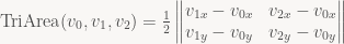
The other standard formula for triangle area is , where b is the length of the base of the triangle (=length of one of its edges) and h is the corresponding height (=length of the perpendicular of b through the vertex opposite b). In fact, the proof for this formula uses the same parallelogram we just saw. Compare the two expressions and we note that our signed area computation can be written

where h(v₂, v₀v₁) denotes the signed height of v₂ over v₀v₁ – this isn’t standard notation, but bear with me for a minute. The point here is that the value of this signed area computation is proportional to the signed distance of v₂ from the edge. That this works on triangles should not be surprising – the same is true for rectangles, for example – but it’s worth spelling out explicitly here because we’ll be doing a lot of signed area computations to determine what is in effect signed distances. So it’s important to know that they’re equivalent.

Edge functions

Now, let’s get back to our original use for these determinant expressions: figuring out on which side of an edge a point lies. So let’s pick an arbitrary point p and see how it relates to the edge v₀v₁. Throwing it into our determinant expression:

and if we rearrange terms a bit, regroup and simplify we get

This is what I’ll call the edge function for edge v₀v₁. As you can see, if we hold the vertex positions constant, this is just an affine function on p. Doing the same with the other two edges gives us two more edge functions:

If all three of these are positive, p is inside the triangle, assuming the triangle is wound counter-clockwise, which I will for the rest of this article. If it’s clockwise, just swap two of the vertices before you start hit-testing. Now, these are normal linear functions, but from their derivation and the determinant properties we saw earlier, we know that they in fact also measure the signed area of the corresponding parallelogram – which in turn is twice the signed area of the corresponding triangle. Let’s pick a point inside the triangle and draw the corresponding diagram:

Our original triangle is partitioned into three smaller triangles that together exactly cover the area of the original triangle. And since p is inside, these triangles are all wound counter-clockwise themselves: they must be, because these triangles have signed areas corresponding to the edge functions, and we know all three of them are positive with p inside. So that’s pretty neat all by itself.

But wait, there’s more! Since the three triangles add up to the area of the original triangle, the three corresponding edge functions should add up to twice the signed area of the full triangle v₀v₁v₂ (twice because triangle area has the 1/2 factor whereas our edge functions don’t). Or, as a formula:

If you look at the terms in the edge functions containing p_x and p_y that shouldn’t be surprising: Summing the three terms for p_x gives (v_0y – v_1y + v_1y – v_2y + v_2y – v_0y) = 0, and similar for p_y. So yes, the sum of these three is constant alright. Now, looking at this in linear algebra terms, this shouldn’t come as a surprise: we have 3 affine functions on only 2 variables – they’re not going to be independent. But it still helps to see the underlying geometry.

Why signed areas are a good idea

Note that the statement about the edge functions summing up to the area of the triangle hold for any point, not just points inside the triangle. It’s not clear how that’s going to work when p is outside the triangle, so let’s have a look:

This time, the triangles actually overlap each other: The two triangles v₀v₁p and v₁v₂p are wound counter-clockwise and have positive area, same as before – also, they extend outside the area of the original triangle. But the third (red) triangle, v₂v₀p, is wound clockwise and has negative area, and happens to exactly cancel out the parts of the two other triangles that extend outside the original triangle v₀v₁v₂. So it still all works out. If you haven’t seen this before, this kind of cancelling is an important trick, and can be used to simplify a lot of things that would otherwise be pretty hairy. For example, it can be used to calculate the area of any polygon, no matter how complicated, by just summing the areas of a bunch of triangles, one triangle for each edge. Doing the same using only positive-area triangles requires triangulating the polygon first, which is a much hairier problem, but again, I digress.

So where’s the barycentric coordinates already?

Now, this blog post is called “the barycentric conspiracy”, but strangely, this far in, we don’t seem to have seen a single barycentric coordinate yet. What’s up with that? Well, let’s first look at what barycentric coordinates are: in the context of a triangle, the barycentric coordinates of a point are a triple (w₀, w₁, w₂) of numbers that act as “weights” for the corresponding vertices. So the three coordinate triples (1,0,0), (0,1,0) and (0,0,1) correspond to v₀, v₁ and v₂, respectively. More generally, we allow the weights to be anything (except all zeros) and just divide through by their sum in the end. Then the barycentric coordinates for p are a triple (w₀, w₁, w₂) such that:

Since we divide through by their sum, they’re only unique up to scale – much like the homogeneous coordinates you’re hopefully familiar with as a graphics programmer. This is the second time we’ve accidentally bumped into them in this post. That is not an accident. Barycentric coordinates are a type of homogeneous coordinates, and in fact both were introduced in the same paper by Möbius in 1827. I’m trying to stick with plain planar geometry in this post since it’s easier to draw (and also easier to follow if you’re not used to thinking in projective geometry). That means the whole homogeneous coordinate angle is fairly subdued in this post, but trust me when I say that everything we’ve been doing in here works just as well in projective spaces. And you’ve already seen the geometric derivations for everything, so we can even do it completely coordinate-free if we wanted to (always good to know how to avoid the algebra if you’re not feeling like it).

But back to barycentric coordinates: We already know that our edge functions measure (signed) areas, and that they’re zero on their respective edges. Well, both v₀ and v₁ are on the edge v₀v₁ (obviously), and hence

.

And we also already know that if we plug the third vertex into the edge function, we get twice the signed area of the whole triangle:

.

The same trick works with the other two edge functions: whenever all three vertices are involved, we get twice the signed area of the whole triangle, otherwise the result is zero. And we already know they’re affine functions. At this point, things should already look fairly suspicious, so I’m just gonna cut to the chase: Let’s set

That’s right, the three edge functions, evaluated at p, give us p’s barycentric coordinates, normalized so their sum is twice the area of the triangle. Note that the barycentric weight is always for the vertex opposite the edge we’re talking about. Now that you’ve seen the area diagram, it should be clear why: what the edge function F₁₂(p) gives us is the scaled area of the triangle v₁v₂p, and the further p is from edge v₁v₂, the larger that triangle is. At the extreme, when p is at v₀, it covers the entirety of the original triangle we started out with. So that all makes sense. While we’re at it, let’s also define a normalized version of the barycentric coordinates with their sum always being 1:

So the secret is out – the determinants we’ve been looking at, the signed areas and distances, even the edge functions – it was barycentric coordinates all along. It’s all connected, and everybody’s in on it! Cue scare chord.

Barycentric interpolation

And with that, we have all the math we need, but there’s one more application that I want to bring up: As I’ve said before, the barycentric coordinates are effectively weights for the various vertices. The definition uses this for the positions, but we can use those same weights to interpolate other stuff that’s supposed to vary linearly across a triangle, such as vertex attributes.

Now, for the depth buffer rasterizer that we’re going to look at, we only need to interpolate one thing, and that’s depth. If we have z values z₀, z₁, z₂ at the vertices, we can determine the interpolated depth by computing

and if we have the edge function values for p already, that’s fairly straightforward and works just fine, at the cost of three multiplies and two adds. But remember that we have the whole thing normalized so the lambdas sum to 1. This means we can express any lambda in terms of the two others:

Plugging this into the above expression and simplifying, we get:

The differences between the z_i‘s are constant across the triangle, so we can compute them once. This gives us an alternative barycentric interpolation expression that uses two multiplies and two adds, in a form that allows them to be executed as two fused multiply-adds. Now if there’s one thing we’ve seen in the previous posts in this series, it’s that counting operations is often the wrong way to approach performance problems, but this one simplification we will end up using in an inner loop that’s actually bottlenecked by the number of instructions executed. And, just as importantly, this is also the expression that GPUs normally use for vertex attribute interpolation. I might talk more about that at some point, but there’s already more than enough material for one sitting in this post. So see you next time, when we learn how to turn all this into a rasterizer.

Frustum culling: turning the crank

This post is part of a series – go here for the index.

In the past few posts, we’ve been looking at Intel’s Software Occlusion Culling sample. This post is going to be a bit shorter than the others so far. This has two reasons: first, next up is the rasterizer. It turns out there’s another common performance problem we’re gonna see in this series, but right now, fixing it is not going to make much of a difference: as it is, the rasterizer in the sample is fairly well balanced, and it’s not making any serious mistakes. In other words, this time round, we don’t get any easy pickings. Unlike the somewhat peripheral framework code we’ve been looking at so far, this is the actual heart of this sample, and it was written by people who know what they’re doing. Speeding it up is going to take some actual algorithmic improvements, which means a lot of prep work for me, since I’ll need to teach you the necessary groundwork first. :) This is gonna take several posts, but I promise that we’ll get a properly satisfying finale.

Well, that’s the first reason. The second reason is that I’ve actually had people complain about the rate at which I’m posting these, because they’re falling behind on reading! Sheesh. You slackers – try writing the damn things! :) Anyway, I’m going to give you this one for the road, and then I’m gonna stop for the weekend so you can catch up and I can start mentally preparing for the figures on rasterization I’m gonna have to produce. A picture may be worth a thousand words, but making a decent illustration takes me a lot longer than writing a thousand words does, so it’s not a happy trade-off.

Anyway, enough introduction. One final batch of frustum cull optimization coming right up. Let’s get cracking.

What we need here is some work ethic

So the whole point of my last post was that you can often make a big difference with fairly small changes, provided you know what you’re doing – minimally invasive surgery, so to speak. This has lots of advantages: it’s easy to write and review, very testable, and less likely to cause major disruptions or cause friction with other existing code. When we last saw our frustum culling code, we managed to speed it up by a factor of over 4.5x by a handful of fixes, none of which touched more than 3 lines of code. That’s both satisfying and impressive to family and friends (if you have the kind of family which tends to be impressed by these things), and it got us from a #4 location in our hot spot list all the way down to #10:

But as you can see, while that blue bar denoting Level-3 cache misses has gotten considerably shorter, it’s still there, and a lot of the things I mentioned in the previous part are still true: in particular, one instance of our TransformedAABBoxSSE is still well above the size of a cache line, and while we’ve managed to beat it all into a shape where the prefetcher works for us, we’re still only accessing 25 bytes per cache line, best case. That’s over 60% of our memory bandwidth wasted. Surely, we can do better?

Well, of course we can, but this time we’re gonna have to roll up our sleeves and do some more invasive changes to our code. Let’s first recap the struct layout:

class TransformedAABBoxSSE
{
    // Methods elided

    CPUTModelDX11 *mpCPUTModel;
    __m128 *mWorldMatrix;
    __m128 *mpBBVertexList;
    __m128 *mpXformedPos;
    __m128 *mCumulativeMatrix; 
    bool   *mVisible;
    float   mOccludeeSizeThreshold;
    __m128 *mViewPortMatrix; 

    float3 mBBCenter;
    float3 mBBHalf;
    bool   mInsideViewFrustum;
    bool   mTooSmall;
    float3 mBBCenterWS;
    float3 mBBHalfWS;
};

The part we care about right now is at the bottom: The two bools and the world-space bounding box. Now, it turns out that while one of the bools (mTooSmall) gets written by the function TransformedAABBoxSSE::IsTooSmall, nobody ever reads it – everyone just uses the return value of IsTooSmall. So we can just make it a local variable in that function and stop spending per-instance memory on it. That one’s fairly easy.

Ta data rhei

For mInsideViewFrustum though, we’re going to have to work a bit more. In particular, we’re gonna have to understand the actual dataflow patterns to figure out where the right place to put it is.

We already know that it gets set in IsInsideViewFrustum, because we’ve spent some time looking at that function already, although it’s gotten shorter since we last saw it:

void TransformedAABBoxSSE::IsInsideViewFrustum(CPUTCamera *pCamera)
{
    mInsideViewFrustum = pCamera->mFrustum.IsVisible(mBBCenterWS,
        mBBHalfWS);
}

Unfortunately, unlike the previous case, IsInsideViewFrustum doesn’t have a return value, so our boolean flag is actual state, and there’s two more methods that access it, one of which is also called IsInsideViewFrustum. I’m really not a fan of overloading when the two methods do completely different things – it’s confusing and error-prone – but I digress. Both of the other methods are inline:

inline void SetInsideViewFrustum(bool insideVF)
{
    mInsideViewFrustum = insideVF;
}

inline bool IsInsideViewFrustum()
{
    return mInsideViewFrustum;
}

And both of these get called from the outside, so we can’t simply nuke them. However, lucky for us, these dependencies don’t go very far upstream in the call graph at all. So let’s have a look where our three frustum cull-related functions get called. First, the function that updates our visibility state. Turns out there’s only two callers. Let’s look at the first one:

void AABBoxRasterizerSSEST::IsInsideViewFrustum(CPUTCamera *pCamera)
{
    mpCamera = pCamera;
    for(UINT i = 0; i < mNumModels; i++)
    {
        mpTransformedAABBox[i].IsInsideViewFrustum(mpCamera);
    }
}

Straightforward enough. The second one is in the class AABBoxRasterizerSSEMT, which does the exact same thing with some additional setup to figure out which part of the model list each task needs to process (it’s multi-threaded, as the name suggests). Both classes derive from the base class AABBoxRasterizer, which holds a bunch of things common to both the single- and multi-threaded implementations, including the array of TransformedAABBoxSSEs.

Because there’s first a global frustum culling pass on multiple threads, which is only then followed by a second pass that looks at the results, we can’t simply get rid of the per-model bookkeeping: it’s actual state. Let’s look at the callers of the no-parameters version of IsInsideViewFrustum to figure out where that state is read:

void AABBoxRasterizerSSEST::TransformAABBoxAndDepthTest()
{
    mDepthTestTimer.StartTimer();

    for(UINT i = 0; i < mNumModels; i++)
    {
        mpVisible[i] = false;
        mpTransformedAABBox[i].SetVisible(&mpVisible[i]);
	
        if(mpTransformedAABBox[i].IsInsideViewFrustum() &&
           !mpTransformedAABBox[i].IsTooSmall(
               mViewMatrix, mProjMatrix, mpCamera))
        {
            mpTransformedAABBox[i].TransformAABBox();
            mpTransformedAABBox[i].RasterizeAndDepthTestAABBox(
                mpRenderTargetPixels);
        }		
    }
    mDepthTestTime[mTimeCounter++] = mDepthTestTimer.StopTimer();
    mTimeCounter = mTimeCounter >= AVG_COUNTER ? 0 : mTimeCounter;
}

And again, there’s a multi-threaded version that does pretty much the same, and no other callers.

Finally, searching for callers to SetInsideViewFrustum turns up exactly one hit, an inline function in AABBoxRasterizerSSE:

inline void ResetInsideFrustum()
{
    for(UINT i = 0; i < mNumModels; i++)
    {
        mpTransformedAABBox[i].SetInsideViewFrustum(true);
    }
}

As far as dataflow expeditions go, this one was pretty much as tame as it gets: it’s all concentrated in a few source files, among functions that are directly related and are at similar levels of the call tree. Refactoring this won’t be hard at all. Mind you, this is pretty much the best-case result – we got off lightly. In a lot of codebases, doing this kind of thing will quickly lead you to realize that the banana you’re interested in and the gorilla holding it are very tightly coupled. But now that we’ve determined that’s not the case, how do we rearrange things for better cache efficiency?

Shuffling data around

As we just saw, AABBoxRasterizerSSE and its subclasses are clearly in charge of running the whole frustum culling operation. Not only do they trigger the frustum culling computation, they also hold the array of bounding boxes, and they’re the only ones who actually look at the frustum culling results. That suggests that AABBoxRasterizerSSE is the natural place to put our frustum calling state. So let’s add an array of bools for the visibility state of the boxes, and make it parallel to the array we already have:

class AABBoxRasterizerSSE : public AABBoxRasterizer
{
  // ...
  TransformedAABBoxSSE *mpTransformedAABBox;
  bool *mpBBoxVisible; // <--- this is new
  // ...
};

This needs to be allocated and freed, but all of that is perfectly routine, so I won’t go into it. And once we’ve added it, we have a fairly simple plan of attack:

• Replace all calls to mpTransformedAABBox[i].IsInsideViewFrustum() (the version without arguments) by mpBBoxVisible[i].
• Similarly, replace calls to SetInsideViewFrustum by the corresponding assignment.
• Instead of writing the culling state to a member variable, have IsInsideViewFrustum(camera) (the update version) return the frustum culling state, and write it to the corresponding slot in mpBBoxVisible at the call site.
• Get rid of TransformedAABBoxSSE::mInsideViewFrustum now that it’s unreferenced.

Each of these items results in a handful of changes; the complete diff is here, for the curious.

And presto, we have a densely packed visibility state array (well, not that densely packed, since we still use a whole byte to store what’s effectively a 1-bit flag, but you get the idea). By itself, that won’t buy us much in the frustum culling pass, although it’s likely to make the later pass that checks for visible boxes faster, since we now never need to fetch the whole TransformedAABBoxSSE from memory if it was frustum culled.

But we can now turn the crank one more time and do the same with the world-space bounding boxes, creating yet another array held by AABBoxRasterizerSSE. We also move the actual visibility test to AABBoxRasterizerSSE (since the test function is a one-liner, that’s a simple change to make), wrap it inside a loop (since we’re always going to be culling a group of models), and call it from the two original frustum-culling loops in the single-threaded and multi-threaded rasterizer variants with the correct loop bounds. All of this is in this commit – as you can see, again it turns out to be mostly small changes.

Finally, for bonus points, we do some cleanup and remove the now-unnecessary fields and methods from TransformedAABBoxSSE. That’s in this commit.

And just like that, we have our bounding boxes densely packed in a nice linear array, and the output visibility flags densely packed in another array. No more reading a whole cache line to only use 25 bytes – this time, we look at everything in the cache lines we access, and we access it all sequentially. That should result in better cache hit rates, lower memory bandwidth usage, and generally better performance. But how much does it actually buy us? Let’s find out!

Whoa – almost down to a third of what we had before we started (for the record, the last few times, I’ve tried to keep run lengths roughly consistent so we can actually compare the cycles directly). Our CPI rate is done below 0.5 – meaning we run at over two instructions executed per clock cycle, sustained, through the whole loop. Those pesky L3 cache misses? Gone completely. And we seem to be surrounded by a lot of functions we haven’t seen before in this series, because by now we’re at rank 20 in the hot spots list – down by another 10 positions! (But wait, is that tan() right below us? What the hell is that doing there… ah well, never mind).

When people tell you that you should optimize for cache usage patterns above all else, this is what they mean.

Well, even before we started, the frustum culling performance was good enough that there was no pressing need to deal with it immediately. At this point, it’s fast enough that we should really focus our attention elsewhere; there are bigger fish to fry. But then again… we seem to be on a winning streak, so why stop now? Let’s aim for some extra credits and see if we can push it a bit further.

Up To Eleven

Now, since I’m cropping the screenshots heavily to make them fit in the blog layout, you can’t see what I see. For all the screen shots we’ve seen so far, I’ve always made the columns narrow and sorted them so that whatever I want to show you happens to be next to the labels. But what you actually get out of the “General Exploration” analysis I’ve had VTune run is more than 20 columns worth of various counters. So for most of the functions on the screen, there’s a bunch of other blue bars and counters that I haven’t shown you, representing various kinds of bottlenecks.

So you can’t see what I see, namely: absolutely nothing next to CalcInsideFrustum. In short, there’s nothing significant left to be gained by modifying data layout or implementation details. This code runs as smoothly as code can be expected to run. If we want to make things go faster still, we actually have to do less work.

Luckily, there’s still one source of inefficiency in the current algorithm: we pass in one box at a time, and test it against all 6 frustum planes. Now, this code uses SSE to test against 4 planes simultaneously, so it’s a fairly decent implementation. But the second half of the test only gives us 2 more planes; the other 2 SIMD lanes are wasted.

This can be fixed by turning the packing around: instead of testing one box against groups of four planes at a time, we test groups of four boxes against one plane at a time. Because we have a lot more boxes than we have planes, that means we have a lot less wasted work overall, at least potentially: the old test always checks one box against 8 planes, of which we actually care about 6. That means 6/8=75% of the computations done are useful. If we instead test groups of four boxes at a time, we run at perfect utilization except for the very last group, which might have less than 4 boxes in it if our total number of boxes is not divisible by four.

Of course, to do this, we need to reorder our box structures so we can grab those four boxes efficiently. Given that the original goal of this post was to be shorter than the other ones and I’m already above 2300 words, I’m not going to delve into the details here, but again, you can just look at the code. So, does it help?

You bet. In fact, if you compare the numbers, we come pretty close to the 1.33x speedup you would expect when increasing utilization from 75% to near 100%. However, as you can see, our clocks per instruction went up again, and our L3 misses. That’s because we’re now starting to outrun the cache prefetching again.

Now, I have a processor with AVX support, and if we were compute limited, we could try use 8-wide SIMD instead of 4-wide SIMD. But considering that we already seem to be processing data faster than we can fetch it, there’s not much point to it. I tried it anyway to be certain, and sure enough, it’s really mostly a way of turning code with slightly too little computation per data item into code with far too little computation per data item. Now given what I saw in that code, I believe that things might look slightly differently in x64 mode, where we get 8 more YMM registers that this code could really make great use of, but I didn’t look into it; this post has gone on for long enough already.

Conclusions

I still stand by what I said in my previous post, namely that you don’t need to go full-on Data-Oriented Design to get good performance on modern CPUs. But all that said, if you’re willing to put in the effort, it definitely does pay off: we got a 3.33x speedup on code that was already using SSE to begin with. Stop counting ALU cycles, people. As this series should have shown you by now, it’s really not so much about what happens when your code runs – it’s about getting rid of the things that make it grind to a halt. As you just saw, data density makes a huge difference in cache efficiency (and hence execution times), and the widest ALUs in the world won’t do you any good if you can’t keep them fed.

And on that note, I’m gonna let this particular pipeline drain over the weekend so you have some time to let it all settle :). See you next time!

Fixing cache issues, the lazy way

This post is part of a series – go here for the index.

Last time, we ended on a bit of a cliffhanger. We’ll continue right where we left off, but first, I want to get a few things out of the way.

First, a lot of people have been asking me what profiler I’ve been using for the various screenshots. So, for the record, the answer is that all these measurements were done using the current version of Intel VTune. VTune has a bit of a learning curve, and if I just want to quickly figure out why something is slow I prefer other tools. But if you’re trying to figure out what’s really going on while your code is running, you want something that supports the CPU’s internal event-based sampling counters and can do the proper analysis, and VTune does. If on the other hand you just want to take a quick peek to figure out why something is slow (which is most of the time while you’re not fine-tuning), I suggest you start with Very Sleepy – it’s free, small and easy to use.

Next, some background on why I’m writing this: I do not intend to badmouth the sample project I’ve been using for this series, nor do I want to suggest it’s doing anything particularly stupid. As you might have noticed, both the write-combining issues and the involuntary sharing we saw last post boiled down to two-line fixes in the source. These kinds of things just happen as code gets written and modified, particularly if there’s deadlines involved. In fact, I’m using this example precisely because the problems I’ve found in it are so very typical: I have run into all of these problems before on other projects, and I assume so have most engine programmers who’ve shipped a game. That’s exactly why I think this is worth writing down: so that people who don’t have much optimization experience and are running into performance problems know what to look for.

Third, lest you get a false impression: I’m in a comfortable position here – I spent two weekends (and the equivalent of maybe 3 days worth of full-time work) looking at the code, profiling and tweaking it. And of course, I’m only writing up the changes that worked. You don’t get to see the false starts and all the ideas that didn’t pan out. Nor am I presenting my changes in chronological order: as you can see in the Github repository, in fact I did the SSE version of CPUTFrustum::IsVisible a whole day before I found the sharing issues that were the actual bottleneck. With 20-20 hindsight, I get to present changes in order of impact, but that’s not how it plays out in practice. The whole process is a lot messier (and less deterministic) than it may seem in these posts.

And with all that out of the way, let’s look at cache effects.

Previously…

…we looked at the frustum culling code in Intel’s Software Occlusion Culling sample. The last blog post ended with me showing this profile:

and explaining that the actual issue is triggered by this (inlined) function:

void TransformedAABBoxSSE::IsInsideViewFrustum(CPUTCamera *pCamera)
{
    float3 mBBCenterWS;
    float3 mBBHalfWS;
    mpCPUTModel->GetBoundsWorldSpace(&mBBCenterWS, &mBBHalfWS);
    mInsideViewFrustum = pCamera->mFrustum.IsVisible(mBBCenterWS,
        mBBHalfWS);
}

which spends a considerable amount of time missing the cache while trying to read the world-space bounding box from mpCPUTModel. Well, I didn’t actually back that up with any data yet. As you can see in the above profile, we spend about 13.8 billion cycles total in AABBoxRasterizerSSEMT::IsInsideViewFrustum in the profile. Now, if you look at the actual assembly code, you’ll notice that a majority of them are actually spent in a handful of instructions:

As you can see, about 11.7 of our 13.8 billion cycles are get counted on a mere two instructions. The column right next to the cycle counts is the number of “last-level cache” (L3 cache) misses. It doesn’t take a genius to figure out that we might be running into cache issues here.

The code you’re seeing is inlined from CPUTModel::GetBoundsWorldSpace, and simply copies the 6 floats describing the bounding box center and half-extents from the model into the two provided locations. That’s all this fragment of code does. Well, the member variables of CPUTModel are one indirection through mpCPUModelT away, and clearly, following that pointer seems to result in a lot of cache misses. In turns out that this is the only time anyone ever looks at data from CPUTModel during the frustum-culling pass. Now, what we really want is the 24 bytes worth of bounding box that we’re going to read. But CPU cores fetch data in units of cache lines, which is 64 bytes on current x86 processors. So best case, we’re going to get 24 bytes worth of data that we care about, and 40 bytes of data that we don’t. If we’re unlucky and the box crosses a cache line boundary, we might even end up fetching 128 bytes. And because it’s behind some arbitrary pointer, the processor can’t easily do tricks like automated memory prefetching that reduce the cost of memory accesses: prefetching requires predictable access patterns, and following pointers isn’t very predictable – not to the CPU core, anyway.

At this point, you might decide to rewrite the whole thing to have more coherent access patterns. Now the frustum culling loop actually isn’t that complicated, and rewriting it (and changing the data structures to be more cache-friendly) wouldn’t take very long, but for new let’s suppose we don’t know that. Is there any way incremental, less error-prone way to give us a quick speed boost, and maybe get us in a better position should we choose to change the frustum culling code later?

Making those prefetchers work

Of course there is, or I wouldn’t be asking. The key realization is that the outer loop in AABBoxRasterizerSSEMT::IsInsideViewFrustum actually traverses an array of bounding boxes (type TransformedAABBoxSSE) in order:

for(UINT i = start; i < end; i++)
{
    mpTransformedAABBox[i].IsInsideViewFrustum(mpCamera);
}

One linear traversal is all we need. We know that the hardware prefetcher is going to load that ahead for us – and by now, they’re smart enough to do that properly even if our accesses are strided, that is, we don’t read all the data between the start and the end of the array, but only some of them with a regular spacing. This means that if we can get those world-space bounding boxes into TransformedAABBoxSSE, they’ll automatically get prefetched for us. And it turns out that in this example, all models are at a fixed position – we can determine the world-space bounding boxes once, at load time. Let’s look at our function again:

void TransformedAABBoxSSE::IsInsideViewFrustum(CPUTCamera *pCamera)
{
    float3 mBBCenterWS;
    float3 mBBHalfWS;
    mpCPUTModel->GetBoundsWorldSpace(&mBBCenterWS, &mBBHalfWS);
    mInsideViewFrustum = pCamera->mFrustum.IsVisible(mBBCenterWS,
        mBBHalfWS);
}

Here’s the punch line: all we really have to do is promote these two variables from locals to member variables, and move the GetBoundsWorldSpace call to init time. Sure, it’s a bit crude, and it leads to data duplication, but on the plus side, this is a really easy thing to try – just move a few lines of code around. If it pans out, we can always do it cleaner later. Which leaves the question – does it pan out?

Of course it does – I get to cheat and only write about the changes that work, remember? As you see, now the clock cycles are back in CPUTFrustum::IsVisible. This is not because it’s gotten mysteriously slower, it’s because IsInsideViewFrustum doesn’t copy any data anymore, so IsVisible is the first function to look at the bounding box cache lines now. Which means that it gets billed for those cache misses now.

It’s still not great (I’ve included the Clocks Per Instruction Rate again so we can see where we stand), but we’re clearly making progress: compared to the first profile at the top of this post, which has a similar total cycle count, we’re very roughly twice as fast – and that’s for IsVisible, which includes not just the cache misses but also the actual frustum culling work. Meanwhile, AABBoxRasterizerSSEMT::IsInsideViewFrustum, now really just a loop, has dropped well out of the top 20 hot spots, as it should. Pretty good for just moving a couple of lines of code around.

Order in the cache!

Okay, our quick fix got the HW prefetchers to work for us, and clearly that gave us a considerable improvement. But we still only need 24 bytes out of every TransfomedAABBoxSSE. How big are they? Let’s have a look at the data members (methods elided):

class TransformedAABBoxSSE
{
    // Methods elided

    CPUTModelDX11 *mpCPUTModel;
    __m128 *mWorldMatrix;
    __m128 *mpBBVertexList;
    __m128 *mpXformedPos;
    __m128 *mCumulativeMatrix; 
    UINT    mBBIndexList[AABB_INDICES]; /* 36 */
    bool   *mVisible;
    bool    mInsideViewFrustum;
    float   mOccludeeSizeThreshold;
    bool    mTooSmall;
    __m128 *mViewPortMatrix; 

    float3 mBBCenter;
    float3 mBBHalf;
    float3 mBBCenterWS;
    float3 mBBHalfWS;
};

In a 32-bit environment, that gives us 226 bytes of payload per BBox (the actual size is a bit more, due to alignment padding). Of these 226 bytes, for the frustum culling, we actually read 24 bytes (mBBCenterWS and mBBHalfWS) and write one (mInsideViewFrustum). That’s a pretty bad ratio, and there’s a lot of memory wasting going on, but for the purposes of caching, we only pay for what we actually read, and that’s not much. That said, even though we don’t access it here, the biggest chunk of data in the whole thing is mBBIndexList at 144 bytes, which is just a list of triangle indices for this BBox. That’s completely unnecessary, since that list is going to be the same for every single BBox in the system. So let’s fix that one and reorder some of the other fields so that the members we’re going to access during frustum culling are close by each other (and hence more likely to hit the same cache line):

class TransformedAABBoxSSE
{
    // Methods elided

    CPUTModelDX11 *mpCPUTModel;
    __m128 *mWorldMatrix;
    __m128 *mpBBVertexList;
    __m128 *mpXformedPos;
    __m128 *mCumulativeMatrix; 
    bool   *mVisible;
    float   mOccludeeSizeThreshold;
    __m128 *mViewPortMatrix; 

    float3 mBBCenter;
    float3 mBBHalf;
    bool   mInsideViewFrustum;
    bool   mTooSmall;
    float3 mBBCenterWS;
    float3 mBBHalfWS;
};

Note that we’re writing mInsideViewFrustum right after we read the bounding boxes, so it makes sense to make them adjacent. I put the fields between the object-space and the world-space bounding box simply because the object-space bounding box is reasonably large (24 bytes, about a third of a cache line) and having it between the flags and the box greatly increases our chance of having to fetch two cache lines not one per box.

So, did it help?

Sure did. IsVisible is down to the number 10 spot, and the CPI Rate is down to an acceptable 1.042 clocks/instruction. Now that’s by no means the end of the line, but I want to make this clear: all I did here was factor out one common array to be a shared static const variable, and reorder some class members. That’s it. If you don’t count the initializers for the 36-element index list (which I’ve copied with comments and generous spacing, so it’s a few lines long), we’re talking less than 10 lines of code changed for all the improvements in this post. Total.

In the last few years, there’s been a push by several prominent game developers to “Data-Oriented Design”, which emphasizes structuring code around desired data-flow patterns, rather than the other way round. That’s a sound design strategy particularly for subsystems like the one we’re looking at. It’s also a good guideline for what you want to work towards when refactoring existing code. But the point I want to make here is that even when trying to optimize existing code within its existing environment, you can achieve substantial gains by a sequence of simple, localized improvements. That will only get you so far, but there’s a lot to be said for incremental techniques, especially if you’re just trying to hit a given performance goal in a limited time budget.

And that’s it for today. I might do another post on the frustum culling (I want it gone from the top 10 completely!), or I might turn to the actual rasterizer code next for a change of pace – haven’t decided yet. Until next time!

Cores don’t like to share

This post is part of a series – go here for the index.

Two posts ago, I explained write combining and used a real-world example to show how badly it can go wrong if you’re not careful. The last part was an out-of-turn rant about some string and memory management insanity that was severely hurting the loading times of that same program. That program was Intel’s Software Occlusion Culling sample, which I’ve been playing around with for the last two weekends.

Well, it turns out that there’s even more common performance problems where those two came from. Now, please don’t walk away with the impression that I’m doing this to pick on either Intel or the authors of that sample. What I’m really trying to do here is talk about common performance problems you might find in a typical game code base. Now, I’ve worked on (and in) several such projects before, and every one of them had its share of skeletons in the closet. But this time, the problems happen to be in an open-source example with a permissive license, written by a third party. Which means I can post the code and my modifications freely, a big plus if I’m going to blog about it – real code is a lot more interesting than straw man examples. And to be honest, I’m a lot more comfortable with publicly talking about performance problems in “abstract code I found on the internet” than I would be doing the same with code that I know a friend hammered out quickly two days before trying to get a milestone out.

What I’m trying to say here is, don’t let this discourage you from looking at the actual occlusion culling code that is, after all, the point of the whole example. And no hard feelings to the guys at Intel who went through the trouble of writing and releasing it in the first place!

Our problem of the day

That said, we’re still not going to see any actual occlusion culling performance problems or optimizations today. Because before we get there, it turns out we have some more low-hanging fruit to pick. As usual, here’s a profile – of the rendering this time.

All the functions with SSE in their names relate to the actual depth buffer rasterizer that’s at the core of the demo (as said, we’re gonna see it eventually). XdxInitXopAdapterServices is actually the user-mode graphics driver, the tbb_graphics_samples thing is the TBB scheduler waiting for worker threads to finish (this sample uses Intel’s TBB to dispatch jobs to multiple worker threads), dxgmms1.sys is the video memory manager / GPU scheduler, and atikmdag.sys is the kernel-mode graphics driver. In short, the top 10 list is full of the kinds of things you would expect in an example that renders lots of small models with software occlusion culling.

Except for that spot up at #2, that is. This function – CPUTFrustum::IsVisible – simply checks whether an axis-aligned bounding box intersects the view frustum, and is used for coarse frustum culling before occlusion is even considered. And it’s a major time sink.

Now, instead of the hierarchical callstack profiling I used last time to look at the loading, this profile was made using hardware event counters, same as in the write combining article. I’ve taken the liberty of spoiling the initial investigation and going straight to the counters that matter: see that blue bar in the “Machine Clears” column? That bar is telling us that the IsVisible function apparently spends 23.6% of its total running time performing machine clears! Yikes, but what does that mean?

Understanding machine clears

What Intel calls a “machine clear” on its current architectures is basically a panic mode: the CPU core takes all currently pending operations (i.e. anything that hasn’t completed yet), cancels them, and then starts over. It needs to do this whenever some implicit assumption that those pending instructions were making turns out to be wrong.

On the Sandy Bridge i7 I’m running this example on, there’s event counters for three kinds of machine clears. Two of them we can safely ignore in this article – one of them deals with self-modifying code (which we don’t have) and one can occur during execution of AVX masked load operations (which we don’t use). The third, however, bears closer scrutiny: its official name is MACHINE_CLEAR.MEMORY_ORDERING, and it’s the event that ends up consuming 23.6% of all CPU cycles during IsVisible.

A memory ordering machine clear gets triggered whenever the CPU core detects a “memory ordering conflict”. Basically, this means that some of the currently pending instructions tried to access memory that we just found out some other CPU core wrote to in the meantime. Since these instructions are still flagged as pending while the “this memory just got written” event means some other core successfully finished a write, the pending instructions – and everything that depends on their results – are, retroactively, incorrect: when we started executing these instructions, we were using a version of the memory contents that is now out of date. So we need to throw all that work out and do it over. That’s the machine clear.

Now, I’m not going to go into the details of how exactly a core knows when other cores are writing to memory, or how the cores make sure that whenever multiple cores try to write to a memory locations, there’s always one (and only one) winner. Nor will I explain how the cores make sure that they learn these things in time to cancel all operations that might depend on them. All these are deep and fascinating questions, but the details are unbelievably gnarly (once you get down to the bottom of how it all works within a core), and they’re well outside the scope of this post. What I will say here is that cores track memory “ownership” on cache line granularity. So when a memory ordering conflict happens, that means something in a cache line that we just accessed changed in the mean time. Might be some data we actually looked at, might be something else – the core doesn’t know. Ownership is tracked at the cache line level, not the byte level.

So the core issues a machine clear whenever something in a cache line we just looked at changed. It might be due to actual shared data, or it might be two unrelated data items that just happen to land in the same cache line in memory – this latter case is normally referred to as “false sharing”. And to clear up something that a lot of people get wrong, let me point out that “false sharing” is purely a software concept. CPUs really only track ownership on a cache line level, and a cache line is either shared or it’s not, it’s never “falsely shared”. So “false sharing” is purely a property of your data’s layout in memory; it’s not something the CPU knows (or can do anything) about.

Anyway, I digress. Evidently, we’re sharing something, intentionally or not, and that something is causing a lot of instructions to get cancelled and re-executed. The question is: what is it?

Finding the culprit

And this is where it gets icky. With a lot of things like cache misses or slow instructions, a profiler can tell us exactly which instruction is causing the problem. Memory ordering problems are much harder to trace, for two reasons: First, they necessarily involve multiple cores (which tends to make it much harder to find the corresponding causal chain of events), and second, because of the cache line granularity, even when they show up as events in one thread, they do so on an arbitrary instruction that happens to access memory near the actual shared data. Might be the data that is actually being modified elsewhere, or it might be something else. There’s no easy way to find out. Looking at these events in a source-level profile is almost completely useless – in optimized code, a completely unrelated instruction that logically belongs to another source line might cause a spike. In an assembly-level profile, you at least get to see the actual instruction that triggers the event, but for the reasons stated above that’s not necessarily very helpful either.

So it boils down to this: a profiler will tell you where to look, and it will usually point you to some code near the code that’s actually causing the problem, and some data near the data that is being shared. That’s a good starting point, but from there on it’s manual detective work – staring at the code, staring at the data structures, and trying to figure out what case is causing the problem. It’s annoying work, but you get better at it over time, and there’s some common mistakes – one of which we’re going to see in a minute.

But first, some context. IsVisible is called in parallel on multiple threads (via TBB) in a global, initial frustum-cull pass. This is where we’re seeing the slowdown. Evidently, those threads are writing to shared data somewhere: it must be writes – as long as the memory doesn’t change, you can’t get any memory ordering conflicts.

Here’s the declaration of the CPUTFrustum class (several methods omitted for brevity):

class CPUTFrustum
{
public:
    float3 mpPosition[8];
    float3 mpNormal[6];

    UINT mNumFrustumVisibleModels;
    UINT mNumFrustumCulledModels;

    void InitializeFrustum( CPUTCamera *pCamera );

    bool IsVisible(
        const float3 &center,
        const float3 &half
    );
};

And here’s the full code for IsVisible, with some minor formatting changes to make it fit inside the layout (excerpting it would spoil the reveal):

bool CPUTFrustum::IsVisible(
    const float3 &center,
    const float3 &half
){
    // TODO:  There are MUCH more efficient ways to do this.
    float3 pBBoxPosition[8];
    pBBoxPosition[0] = center + float3(  half.x,  half.y,  half.z );
    pBBoxPosition[1] = center + float3(  half.x,  half.y, -half.z );
    pBBoxPosition[2] = center + float3(  half.x, -half.y,  half.z );
    pBBoxPosition[3] = center + float3(  half.x, -half.y, -half.z );
    pBBoxPosition[4] = center + float3( -half.x,  half.y,  half.z );
    pBBoxPosition[5] = center + float3( -half.x,  half.y, -half.z );
    pBBoxPosition[6] = center + float3( -half.x, -half.y,  half.z );
    pBBoxPosition[7] = center + float3( -half.x, -half.y, -half.z );

    // Test each bounding box point against each of the six frustum
    // planes.
    // Note: we need a point on the plane to compute the distance
    // to the plane. We only need two of our frustum's points to do
    // this. A corner vertex is on three of the six planes.  We
    // need two of these corners to have a point on all six planes.
    UINT pPointIndex[6] = {0,0,0,6,6,6};
    UINT ii;
    for( ii=0; ii<6; ii++ )
    {
        bool allEightPointsOutsidePlane = true;
        float3 *pNormal = &mpNormal[ii];
        float3 *pPlanePoint = &mpPosition[pPointIndex[ii]];
        float3 planeToPoint;
        float distanceToPlane;
        UINT jj;
        for( jj=0; jj<8; jj++ )
        {
            planeToPoint = pBBoxPosition[jj] - *pPlanePoint;
            distanceToPlane = dot3( *pNormal, planeToPoint );
            if( distanceToPlane < 0.0f )
            {
                allEightPointsOutsidePlane = false;
                break; // from for.  No point testing any
                // more points against this plane.
            }
        }
        if( allEightPointsOutsidePlane )
        {
            mNumFrustumCulledModels++;
            return false;
        }
    }

    // Tested all eight points against all six planes and
    // none of the planes had all eight points outside.
    mNumFrustumVisibleModels++;
    return true;
}

Can you see what’s going wrong? Try to figure it out yourself. It’s a far more powerful lesson if you discover it yourself. Scroll down if you think you have the answer (or if you give up).

 

The reveal

As I mentioned, what it takes for memory ordering conflicts to occur is writes. The function arguments are const, and mpPosition and mpNormal aren’t modified either. Local variables are either in registers or on the stack; either way, they’re far enough away between different threads not to conflict. Which only leaves two variables: mNumFrustumCulledModels and mNumFrustumVisibleModels. And indeed, both of these global (debugging) counters get stored per instance. All threads happen to use the same instance of CPUTFrustum, so the write locations are shared, and we have our culprit. Now, in a multithreaded scenario, these counters aren’t going to produce the right values anyway, because the normal C++ increments aren’t an atomic operation. As I mentioned before, these counters are only there for debugging (or at least nothing else in the code looks at them), so we might as well just remove the two increments altogether.

So how much does it help to get rid of two meager increments?

Again, the two runs have somewhat different lengths (because I manually start/stop them after loading is over), so we can’t compare the cycle counts directly, but we can compare the ratios. CPUTFrustum::IsVisible used to take about 60% as much time as our #1 function, and was in the #2 spot. Now it’s at position 5 in the top ten and takes about 32% as much time as our main workhorse function. In other words, removing these two increments just about doubled our performance – and that’s in a function that does a fair amount of other work. It can be even more drastic in shorter functions.

Just like we saw with write combining, this kind of mistake is easy to make, hard to track down and can cause serious performance and scalability issues. Everyone I know that has seriously used threads has fallen into this trap at least once – take it as a rite of passage.

Anyway, the function is now running smoothly, not hitting any major stalls and in fact completely bound by backend execution time – that is, the expensive part of that function is now the actual computational work. As the TODO comment mentions, there’s better ways to solve this problem. I’m not gonna go into it here, because as it turns out, I already wrote a post about efficient ways to solve this problem using SIMD instructions a bit more than two years ago – using Cell SPE intrinsics, not SSE intrinsics, but the idea remains the same.

I won’t bother walking through the code here – it’s all on GitHub if you want to check it out. But suffice to say that, with the sharing bottleneck gone, IsVisible can be made much faster indeed. In the final profile I took (using the SSE), it shows up at spot number 19 in the top twenty.

Two steps forward, one step back

All is not well however, because the method AABBoxRasterizerSSEMT::IsInsideViewFrustum, which you can (barely) see in some of the earlier profiles, suddenly got a lot slower in relation:

Again, I’m not going to dig into it here now deeply, but it turns out that the this is the function that calls IsVisible. No, it’s not what you might be thinking – IsVisible didn’t get inlined or anything like that. In fact, its code looks exactly like it did before. And more to the point, the problem actually isn’t in AABBoxRasterizerSSEMT::IsInsideViewFrustum, it’s inside the function TransformedAABBoxSSE::IsInsideViewFrustum, which it calls, and which does get inlined into AABBoxRasterizerSSEMT::IsInsideViewFrustum:

void TransformedAABBoxSSE::IsInsideViewFrustum(CPUTCamera *pCamera)
{
    float3 mBBCenterWS;
    float3 mBBHalfWS;
    mpCPUTModel->GetBoundsWorldSpace(&mBBCenterWS, &mBBHalfWS);
    mInsideViewFrustum = pCamera->mFrustum.IsVisible(mBBCenterWS,
        mBBHalfWS);
}

No smoking guns here either – a getter call to retrieve the bounding box center and half-extents, followed by the call to IsVisible. And no, none of the involved code changed substantially, and there’s nothing weird going on in GetBoundsWorldSpace. It’s not a virtual call, and it gets properly inlined. All it does is copy the 6 floats from mpCPUTModel to the stack.

What we do have in this method, however, is lots of L3 cache misses (or Last-Level Cache misses / LLC misses, as Intel likes to call them) during this copying. Now, the code doesn’t have any more cache misses now than it did before I added some SSE code to IsVisible. But it generates them a lot faster than it used to. Before, some of the long-taking memory fetches overlapped with the slower execution of the visibility test for an earlier box. Now, we’re going through instructions fast enough for the code to starve waiting for the bounding boxes to arrive.

That’s how it is dealing with Out-of-Order cores: They’re really quite good at making the best of a bad situation. Which also means that often, fixing a performance problem just immediately moves the bottleneck somewhere else, without any substantial speed-up. It often takes several attempts to tackle the various bottlenecks one by one until, finally, you get to cut the Gordian Knot. And to get this one faster, we’ll have to improve our cache usage. Which is a topic for another post. Until next time!